Lecture 7 · Policy Gradient

Slides: David Silver - RL Course (UCL 2015) · Previous: Lecture 6 · Value Function Approximation · Next: Lecture 8 · Integrating Learning and Planning

First pass: read The one idea and the slide-group headings. Use the prose when an equation, condition, or figure needs explanation; leave Gaps to close for review.

Highlights: definition or core claim · intuition, mechanism, how to read · Silver's own words · caveat or condition.

The video's deck is a later version than this PDF

Two differences that matter, both confirmed by watching the timestamps against the pages:

The video teaches the deterministic policy gradient (⏱ 1:26:32–1:29:36). No slide for it exists in this deck. It is covered in 9 · What the deck does not have below.
The deck's p.35–37 (natural policy gradient) is explicitly skipped in the video, along with the p.38–40 snake demo that illustrates it.
The video moves compatible function approximation to ⏱ 1:23:27, after the baseline and trace material. This note keeps the PDF's p.26→p.34 order, so the timestamps in section 8 intentionally jump backward.

Notation also drifted: the video says $u$ for actor parameters and $v$ for critic parameters; this deck says $\theta$ and $w$ / $v$ . This note uses the deck's $\theta$ throughout, since the deck is what is embedded here.

The one idea

L6 parameterized the value function and then read a policy off it with $\arg\max_a$ . L7 deletes that step: parameterize the policy directly, $\pi_\theta(s,a)=\mathbb{P}[a\mid s,\theta]$ , and push $\theta$ uphill on reward.

Once you do, the entire lecture collapses into one equation with one swappable slot:

\nabla_\theta J(\theta)=\mathbb{E}_{\pi_\theta}\Big[\underbrace{\nabla_\theta\log\pi_\theta(s,a)}_{\text{how to do more of this action}}\times\underbrace{\;?\;}_{\text{was it any good}}\Big]

Every algorithm in the lecture chooses a different learning signal for the second factor:

Signal	Algorithm	What changes
$G_t$ (the sampled return)	REINFORCE	unbiased return estimate, usually high variance
$Q_w(s,a)$	Q actor-critic	lower-variance learned critic; approximation can bias the update
$A_w(s,a)$	advantage actor-critic	subtracts a baseline so only relative action quality remains
$\delta_t$ (TD error)	TD actor-critic	one-step online signal using only a $V$ -critic
$\delta_t e_t$ (trace)	TD( $\lambda$ ) actor-critic	mixes credit over multiple time-scales

That table is slide p.41. Everything before it is the derivation of one row.

The max is the problem

Read p.5's advantage list backwards and much of it traces to deleting $\arg\max_a$ . Continuous action spaces are hard for value-based control because the max becomes an optimization problem solved at every step. Approximate greedy improvement can also switch policies abruptly and chatter → L6 p.32.
Policy gradient never computes a max. Silver names this outright as the number-one practical reason to use these methods.

Policy gradient is maximum likelihood, weighted by how well it went

$\nabla_\theta\log\pi_\theta(s,a)$ is exactly the score function from maximum likelihood estimation — the direction that makes the action you took more probable. In supervised learning you would follow it as-is, because a teacher told you $a$ was correct.
RL has no teacher, so it multiplies that same direction by a number saying whether $a$ turned out well. Positive: do more of it. Negative: do the opposite. That is the whole idea, and everything else is variance reduction.

1 · Why parameterize the policy
2 · When you actually need randomness
3 · What best even means
4 · Finite differences
5 · The score function
6 · The policy gradient theorem
7 · Actor-critic
8 · Removing the bias, reducing the variance
9 · What the deck does not have
Study checklist
Gaps to close on your own
Language notes

1 · Why parameterize the policy

p.3–4 · Policy-Based Reinforcement Learning ⏱ 3:05

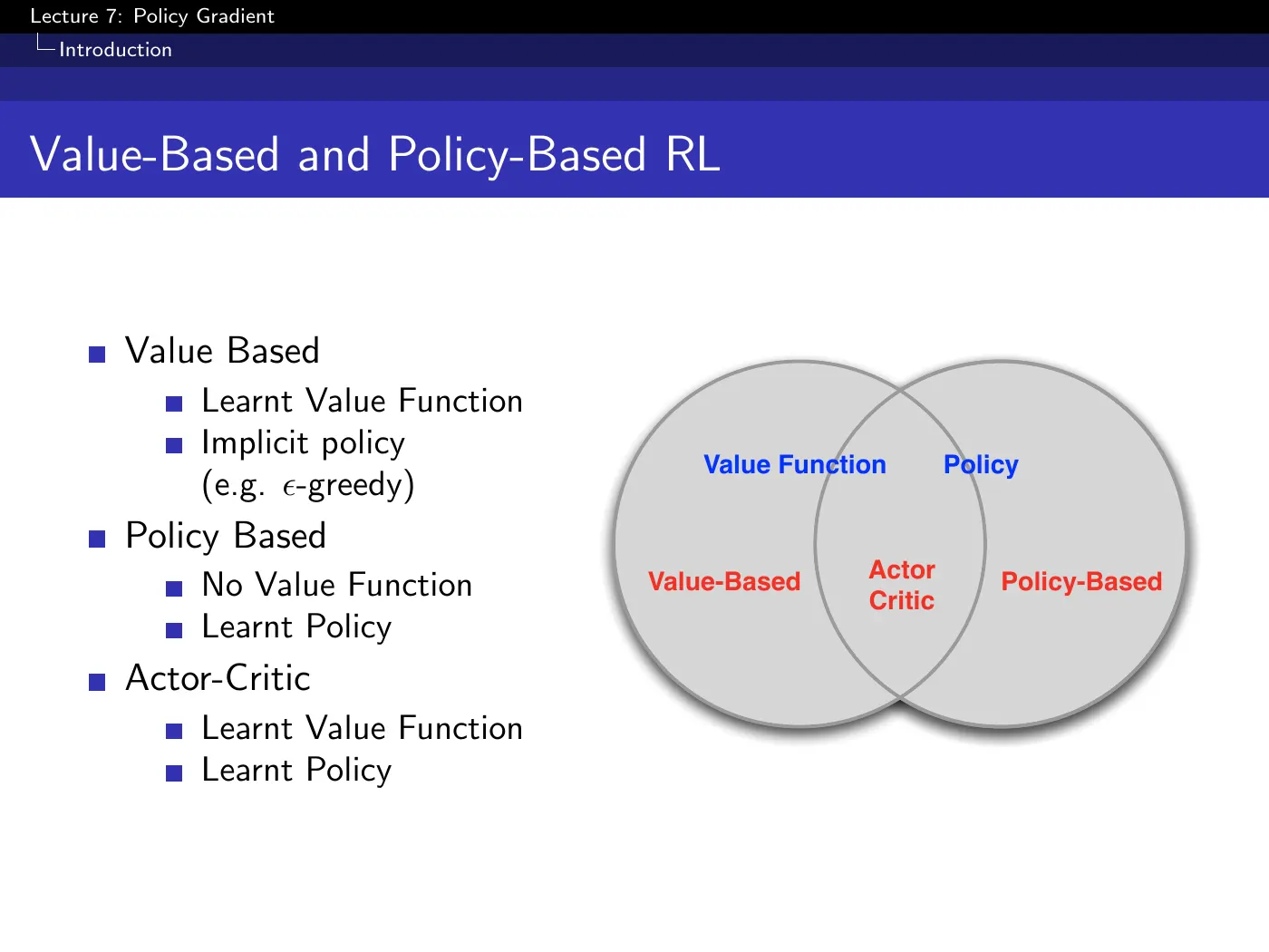
On the surface the change is a letter: L6 fitted $\hat v(s,\mathbf{w})$ , L7 fits $\pi_\theta(s,a)$ . The real change is one of status. In L6 the policy was a derived object — a consequence of the value function plus an $\arg\max$ . Here the policy is the primary object, and the value function becomes optional.

The Venn diagram is worth more than it looks. Three regions, and the middle one is where the rest of the course lives.

There is no ε-greedy on this side of the diagram

$\epsilon$ -greedy is no longer required to turn $Q$ into a behaviour policy, because $\pi_\theta$ is already an explicit policy. Exploration can come from that policy's stochasticity and may be shaped by entropy regularization, parameter noise, or other mechanisms.
The conceptual break from L5 is that randomness can now be state-dependent and learned, rather than imposed as the same uniform perturbation everywhere.

p.5 · Advantages of Policy-Based RL ⏱ 9:20

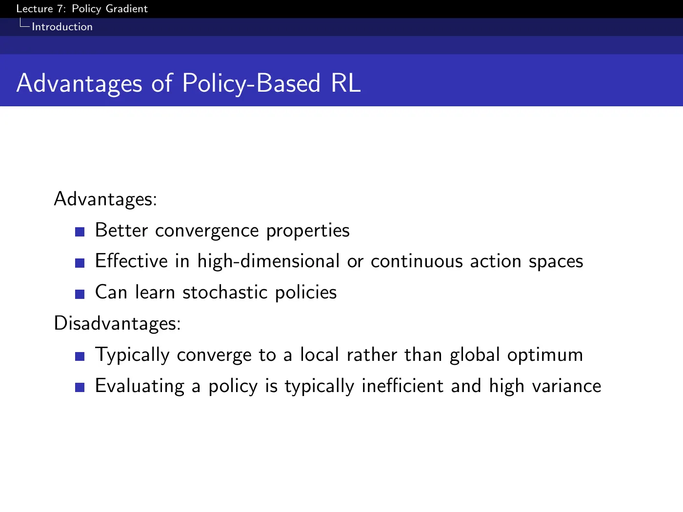
The slide lists three advantages flat. They are not equally important:

Effective in continuous or high-dimensional action spaces. The practical number one. With a trillion actions or a continuous torque vector, $\arg\max_a Q(s,a)$ is an optimization problem you must solve at every time-step. Policy gradient never poses it — it incrementally learns where the max is instead of recomputing it.
Better-behaved policy updates. A gradient step can change the policy smoothly instead of replacing it with a fully greedy policy at once. It can still overshoot with a bad step size and can still settle at a local optimum; the claim is comparative, not absolute.
Can learn stochastic policies. Sometimes necessary, for two separate reasons — p.6 and p.9.

And the disadvantages, restated so they are not just words:

Local rather than global optimum — see the four failed runs on p.22.
Inefficient, high variance — you evaluate a policy by running it and watching what happens, which is noisy. The whole back half of the lecture is variance reduction.

A student's answer that is worth keeping: when is a policy cheaper to represent than a value function?

When the decision is simpler than the evaluation. In Breakout, computing that you will score exactly 1,714 points from here is a hard function to approximate. Encoding "if the ball is coming down over there, move left" may be trivial.
The converse also happens — sometimes the value function is the compact object. Neither representation dominates; it depends on which of the two questions your domain makes easy.

2 · When you actually need randomness

p.6 · Rock-Paper-Scissors ⏱ 14:39

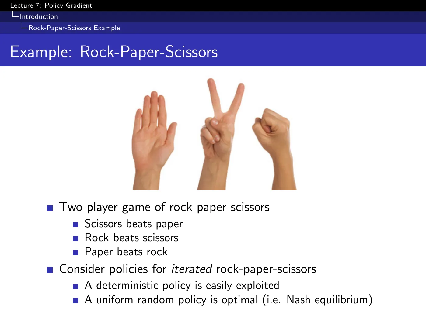
The uniform random policy is the Nash equilibrium, and any deterministic policy is exploited immediately.

The reason matters, because it is not the same reason as the next example. Here the environment contains an adaptive opponent — any regularity in your play becomes a pattern someone else optimizes against. Stochasticity is required by game theory, not by any deficiency in your state representation.

p.7–9 · Aliased Gridworld ⏱ 15:25

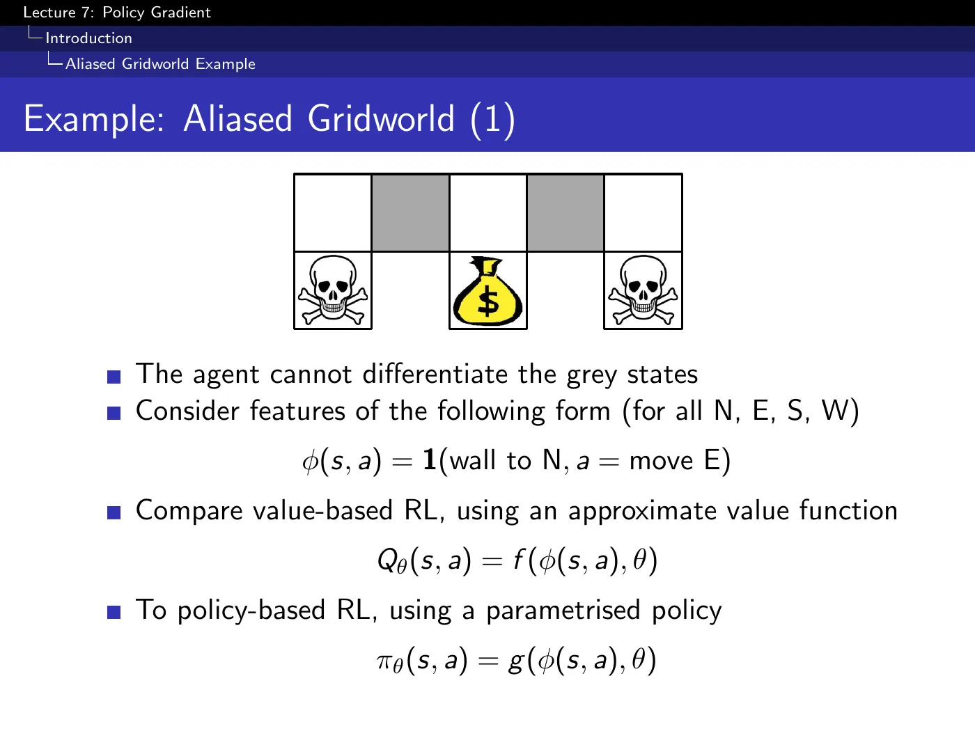
The features are (wall direction, action) pairs, e.g. $\phi(s,a)=\mathbf{1}(\text{wall to N},\,a=\text{move E})$ .

The mechanism, which the slide states as a conclusion rather than an argument: the two grey squares both have a wall to the N and a wall to the S, so their feature vectors are identical. Any function of those features — linear, neural network, your favorite thing — must therefore return the same output for both. It is not that the approximator is too weak. The two states are one state as far as the representation is concerned.

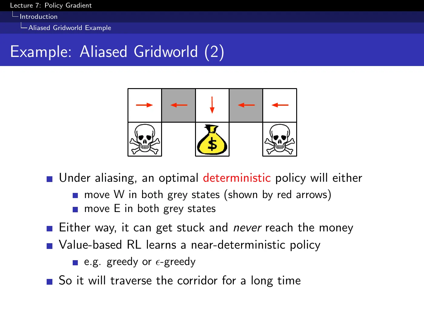
A deterministic policy must then take the same action in both grey squares. Move W in both, and from the right-hand side you oscillate in the corridor and never reach the money. Move E in both, and the same trap appears on the other side.

This does not contradict the theorem from L2

L2 proved that every MDP has a deterministic optimal policy. That result holds under a Markov state representation — full observability, table lookup. Feature aliasing destroys the Markov property, so the problem is effectively a POMDP, and the theorem simply does not apply to it.
Silver makes this dependency explicit. Keep the condition attached to the theorem, because the two statements look contradictory the moment you drop it.

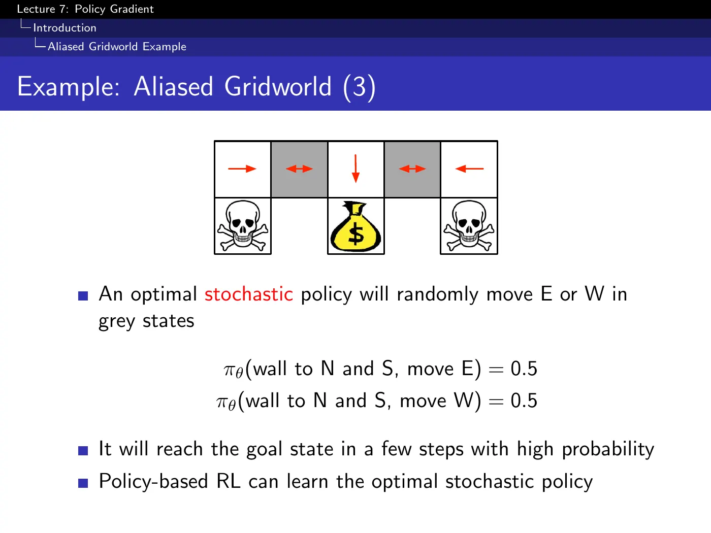
Why ε-greedy cannot rescue this, even though it is stochastic

$\epsilon$ -greedy is random, but its random component is fixed and uniform. A single global $\epsilon$ cannot express “mix 50/50 at this ambiguous observation, but act almost deterministically elsewhere” without unnecessary randomness in the rest of the state space.
A parameterized stochastic policy can learn where to be random and how much. That is the capability this example is meant to isolate. The issue is not that every $\epsilon$ -greedy policy must fail under every tie-breaking rule; it is that the policy class is a poor and inflexible fit for the required behavior.

3 · What best even means

p.10 · Policy Objective Functions ⏱ 20:48

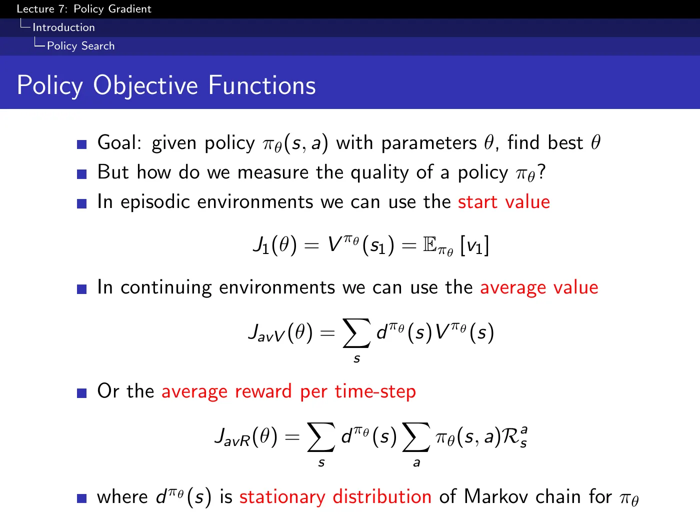
J_1(\theta)=V^{\pi_\theta}(s_1),\qquad J_{avV}(\theta)=\sum_s d^{\pi_\theta}(s)V^{\pi_\theta}(s),\qquad J_{avR}(\theta)=\sum_s d^{\pi_\theta}(s)\sum_a \pi_\theta(s,a)\mathcal{R}^a_s

Three objectives — start value for episodic tasks, average value and average reward for continuing ones.

Choose the objective that matches the task. They are not the same optimization problem and their state-weighting distributions need not be simple rescalings of one another. What is shared is the form of the policy-gradient theorem on p.20: a score function multiplied by a long-term action value, with the appropriate state distribution for the chosen objective.

d^{\pi_\theta}(s)

depends on

\theta

— and that is the hard part

The stationary distribution is written as if it were fixed, but changing $\theta$ changes both the action probabilities and which states you end up visiting. A naive differentiation of $J$ would produce a term in $\nabla_\theta d^{\pi_\theta}$ , and that term is hopeless: it requires knowing how the environment's dynamics respond to a policy change, which is a model.
The policy gradient theorem reorganizes these indirect state-distribution effects into an expectation over visited states; it does not pretend that the state distribution is independent of $\theta$ . That reorganization is why the final estimator can be model-free even though the distribution changes with the policy.

p.11 · Policy Optimization ⏱ 23:49

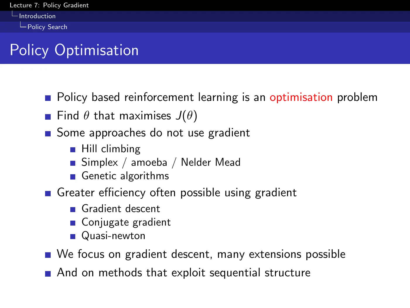
The last bullet is the one that matters and it is easy to skim past: methods that exploit sequential structure.

A genetic algorithm treats a whole lifetime as a single number — run the robot until it dies, get one score, repeat. RL should crack the trajectory open and use the intermediate states and rewards. That is the difference between optimizing a policy and learning within a lifetime, and it is the reason gradient-free methods appear on this slide only to be set aside.

4 · Finite differences

p.12–13 · Computing Gradients By Finite Differences ⏱ 26:52

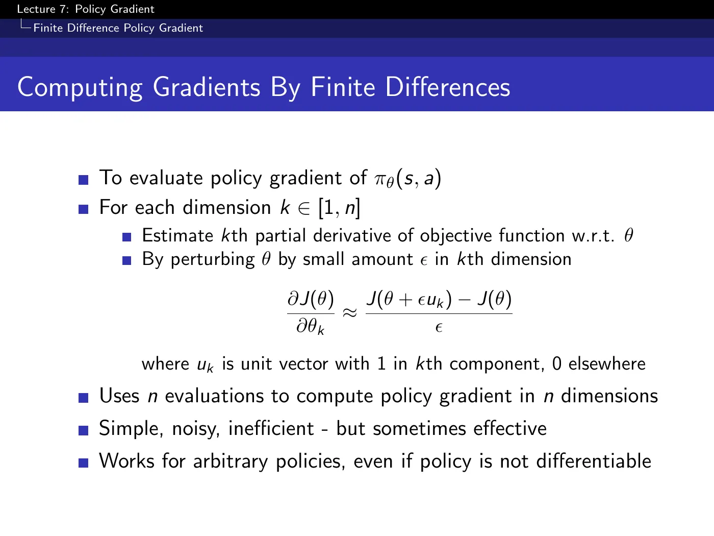
\frac{\partial J(\theta)}{\partial\theta_k}\approx\frac{J(\theta+\epsilon u_k)-J(\theta)}{\epsilon}

Perturb one parameter, re-run the policy, measure the difference. $n$ evaluations for $n$ dimensions — and each "evaluation" means actually running the robot, repeatedly, because the measurement is noisy.

The cost is prohibitive above trivial dimensionality: a neural network with a million parameters would need a million perturbation experiments per gradient step. SPSA and related methods perturb in random directions to cut the count, but the estimates stay very noisy.

The one thing finite differences can do that nothing else here can

It works on non-differentiable policies. If someone hands you a black-box controller with tunable knobs and no derivatives — a hand-written gait, a legacy program, a simulator you cannot backpropagate through — this is still available when every method after this slide is not.
That is why the technique survives despite being obviously inefficient.

p.14–15 · Training AIBO to Walk ⏱ 29:56

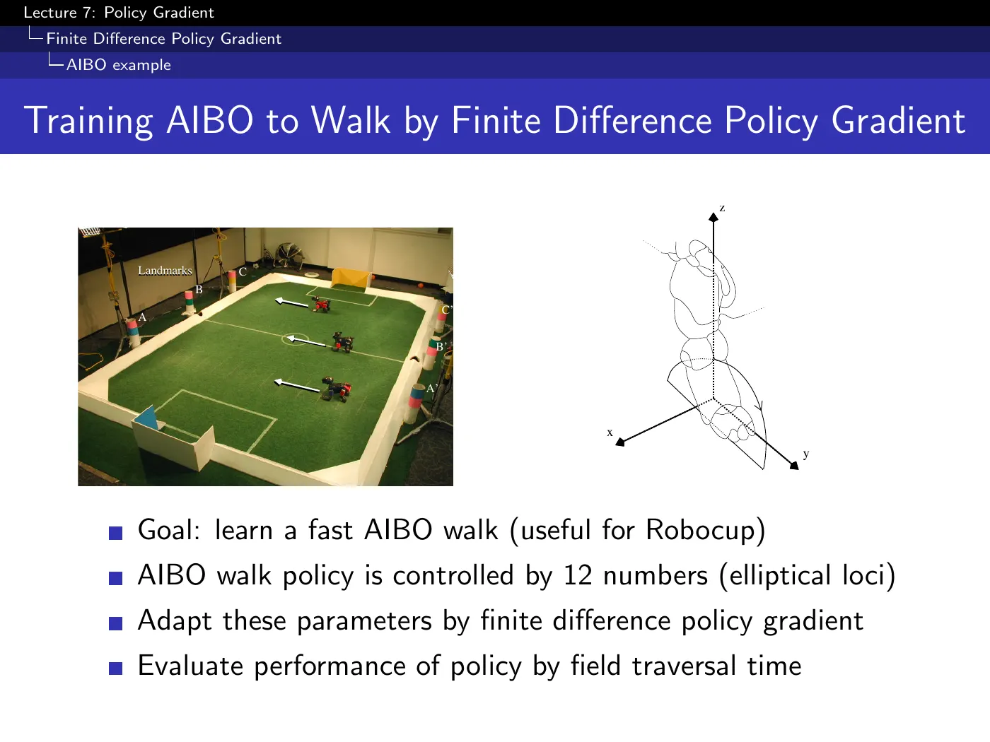
RoboCup's AIBO league was effectively decided by walking speed, so gait optimization became a real machine-learning contest. The gait is 12 real numbers describing half-elliptical foot loci; the objective is measured by timing the robot walking between landmarks.

Work out what one gradient step costs: 12 dimensions, each needing its own perturbed policy, each policy timed over several traversals to average out the noise, all of it in real time on physical hardware. The paper's own figures put one iteration at roughly seven and a half minutes of continuous robot walking.

The before/after videos show what actually improved: the untrained gait slips, and the learned gait is one that copes with the surface friction. The learned parameters beat both hand-tuned gaits and previously learned ones — the method is crude but it was not toy.

5 · The score function

p.16 · Score Function ⏱ 33:45

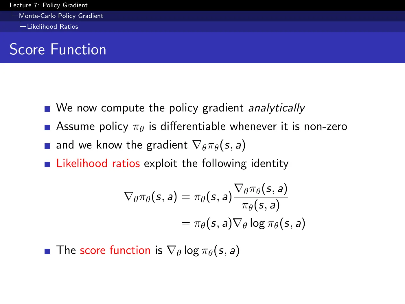
\nabla_\theta\pi_\theta(s,a)=\pi_\theta(s,a)\frac{\nabla_\theta\pi_\theta(s,a)}{\pi_\theta(s,a)}=\pi_\theta(s,a)\,\nabla_\theta\log\pi_\theta(s,a)

Multiply and divide by $\pi_\theta$ . Algebraically trivial, and it is the hinge the entire remaining lecture turns on.

What the trick actually buys

You start with $\nabla_\theta\,\mathbb{E}[\cdot]$ — the gradient of an expectation, which you cannot sample. You finish with $\mathbb{E}[\cdot]$ — an expectation of a gradient, under $\pi_\theta$ , which is the distribution you are already sampling from by acting.
That conversion is why the agent can estimate its own policy gradient from nothing but the trajectory it happens to walk. Whenever $\nabla_\theta\log\pi_\theta$ appears for the rest of the course, this is where it came from.

The score form requires differentiability wherever $\pi_\theta(a\mid s)>0$ . Most textbook derivations therefore use a fixed support with positive probability for the sampled actions; parameter-dependent support or exact zero probabilities need separate care because $\log\pi_\theta(a\mid s)$ is then undefined.

p.17–18 · Softmax and Gaussian Policies ⏱ 36:49

\pi_\theta(s,a)\propto e^{\phi(s,a)^\top\theta} \qquad\Longrightarrow\qquad \nabla_\theta\log\pi_\theta(s,a)=\phi(s,a)-\mathbb{E}_{\pi_\theta}[\phi(s,\cdot)]

a\sim\mathcal{N}(\mu(s),\sigma^2),\quad \mu(s)=\phi(s)^\top\theta \qquad\Longrightarrow\qquad \nabla_\theta\log\pi_\theta(s,a)=\frac{(a-\mu(s))\,\phi(s)}{\sigma^2}

Every score function reads "how much more than usual"

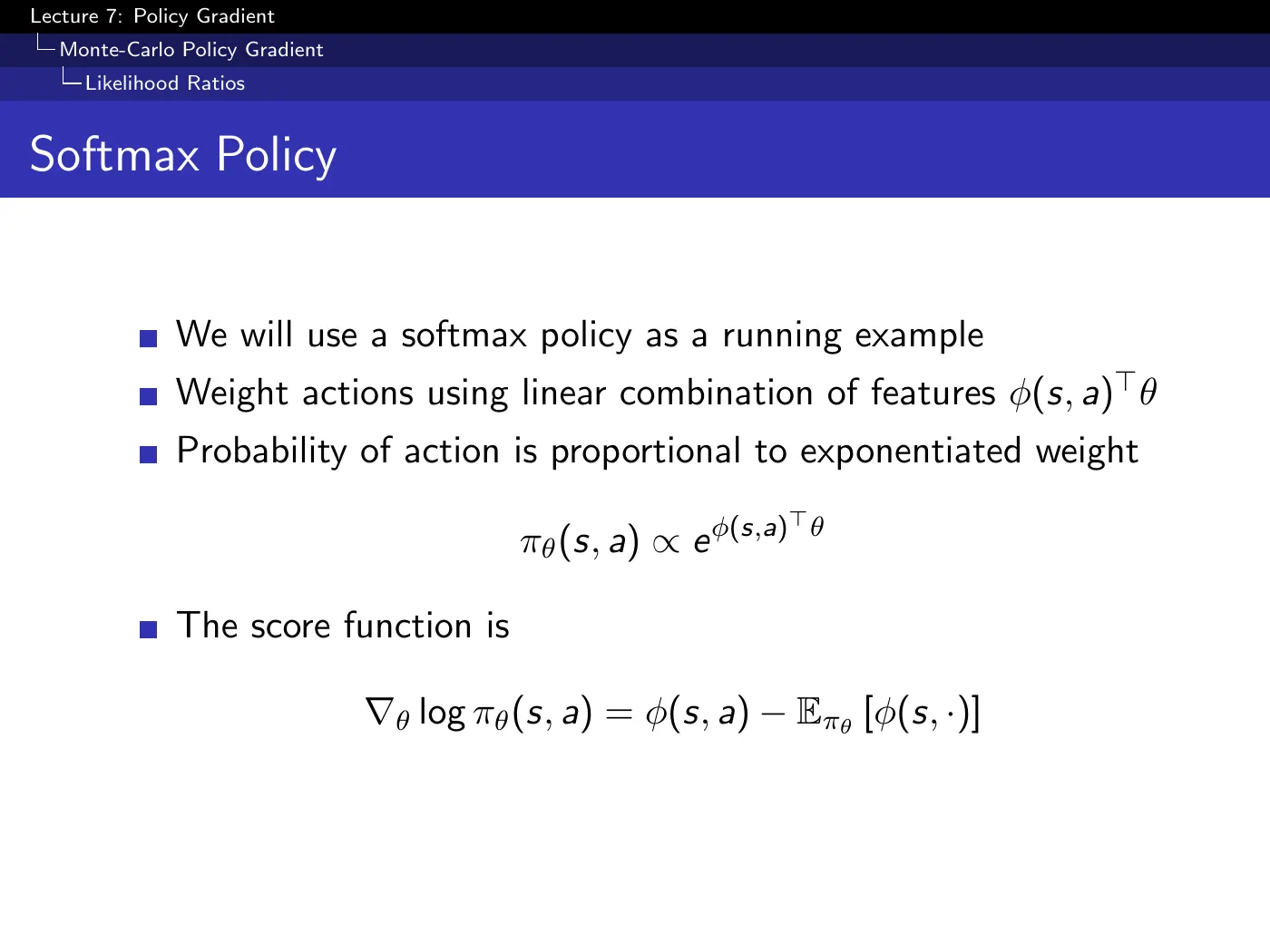
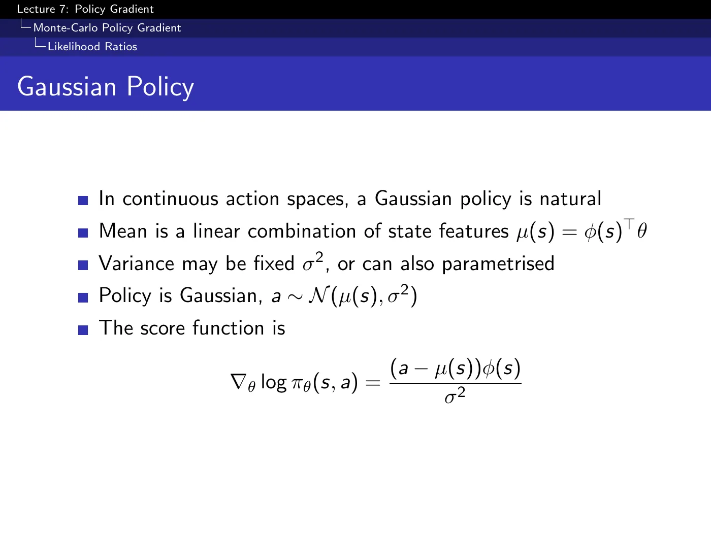
The two examples look unrelated and have the identical shape:

Softmax: (feature of the action I took) − (average feature over actions I might have taken).
Gaussian: (the action I took) − (the action I usually take), times features.

Both are a deviation from your own average behavior. Multiply by "was it good" and the update reads: when something you did more than usual worked out, do more of it. This intuition survives into every algorithm below, and it is why the advantage function on p.29 feels inevitable when it arrives.

Softmax is the discrete-action workhorse; Gaussian is the natural continuous-action choice, which is precisely the case value-based methods could not handle.

6 · The policy gradient theorem

p.19 · One-Step MDPs ⏱ 41:20

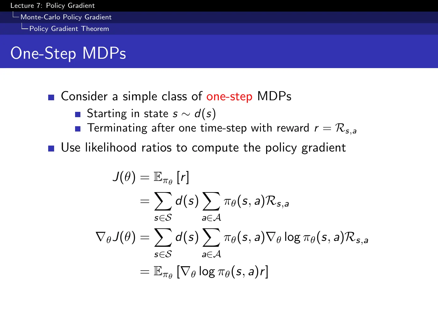
The only derivation given in the lecture, and it is two moves:

J(\theta)=\sum_{s}d(s)\sum_a\pi_\theta(s,a)\mathcal{R}_{s,a}

Only $\pi_\theta$ depends on $\theta$ , so the gradient passes through both sums and lands on $\pi_\theta$ alone.
Apply the likelihood ratio, turning $\nabla_\theta\pi_\theta$ back into $\pi_\theta\nabla_\theta\log\pi_\theta$ — which restores the expectation:

\nabla_\theta J(\theta)=\mathbb{E}_{\pi_\theta}\big[\nabla_\theta\log\pi_\theta(s,a)\,r\big]

A one-step MDP is a contextual bandit, which is where L9 picks this up.

The derivation uses

\mathcal{R}_{s,a}

, the MDP's reward function. Doesn't that make this model-based?

No — and the distinction is worth being precise about. $\mathcal{R}_{s,a}$ is the environment's reward function; $r$ is the reward you actually received. The derivation passes through the function, but the result is an expectation containing only the sampled reward.
So: the derivation refers to the model, the algorithm never does. To take a gradient step you need the score (which you can compute, since $\pi_\theta$ is yours) and the reward you observed. Nothing else. The same pattern recurs on p.31, where a Bellman identity is used to justify a quantity you only ever sample.

p.20 · Policy Gradient Theorem ⏱ 46:41

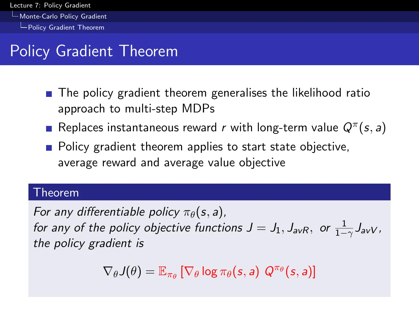
\nabla_\theta J(\theta)=\mathbb{E}_{\pi_\theta}\big[\nabla_\theta\log\pi_\theta(s,a)\,Q^{\pi_\theta}(s,a)\big]

One substitution: the immediate reward $r$ becomes the long-term value $Q^{\pi_\theta}(s,a)$ . That is the entire generalization from one step to many, as far as the final formula is concerned.

The proof is left as an exercise in the lecture. It is short, and worth seeing once, because it shows how the $\nabla_\theta d^{\pi_\theta}$ term flagged at p.10 disappears (Sutton & Barto 2e §13.2, episodic case):

Start from $\nabla v_\pi(s)=\nabla\sum_a\pi(a|s)q_\pi(s,a)$ and apply the product rule: $\sum_a\big[\nabla\pi(a|s)\,q_\pi(s,a)+\pi(a|s)\,\nabla q_\pi(s,a)\big]$ .
Expand the second term with $q_\pi(s,a)=\sum_{s',r}p(s',r|s,a)\big(r+v_\pi(s')\big)$ . This is the key step: $p$ and $r$ belong to the environment, so they do not depend on $\theta$ and the gradient walks straight past them, leaving $\sum_{s'}p(s'|s,a)\nabla v_\pi(s')$ — the same quantity, one state later.
Unroll that recursion. Each step peels off one $\nabla\pi\,q_\pi$ term and hands back another $\nabla v_\pi$ , so repeated substitution gives $\nabla v_\pi(s)=\sum_x\sum_{k=0}^{\infty}\Pr(s\to x,k,\pi)\sum_a\nabla\pi(a|x)q_\pi(x,a)$ .
Set $s=s_0$ . The sum over $k$ counts how often each state is visited, and normalizing it is the on-policy distribution $\mu$ .

The state distribution is never differentiated — it falls out of the recursion

In this proof route, one differentiates $v_\pi$ and recursively expands the effect of future policy choices. The environment's $p(s',r|s,a)$ is constant with respect to $\theta$ , while the visitation weights appear after the recursion is unrolled. The dependence of future state occupancy on the policy has therefore been accounted for, not discarded.
That is exactly why the algorithm comes out model-free — and it is the same structural move as the one-step derivation on p.19: the environment appears in the derivation and is absent from the result.

Equality depends on the state-distribution convention

The deck writes an equality because it chooses objective-specific visitation distributions and, for average value, an explicit scale factor. Other textbooks write the same result with $\propto$ or with an unnormalized discounted occupancy measure. These forms give the same ascent direction after a positive constant is absorbed into $\alpha$ , but their gradient magnitudes are not interchangeable. Always state the objective and occupancy convention before comparing formulas.

Compare it against supervised learning one more time: maximum likelihood would be $\mathbb{E}[\nabla_\theta\log\pi_\theta(s,a)]$ for teacher-supplied actions. RL has no teacher, so it tries actions and weights each by how good $Q$ says it was.

p.21–22 · REINFORCE and Puck World ⏱ 48:13

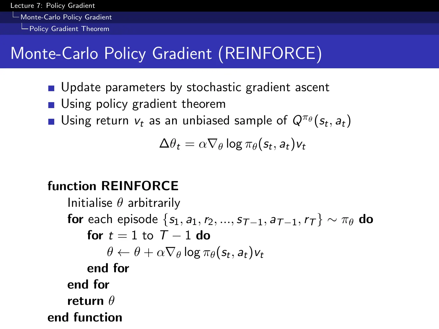
\Delta\theta_t=\alpha\,\nabla_\theta\log\pi_\theta(s_t,a_t)\,v_t

Here the deck's $v_t$ means the sampled return from time $t$ , usually written $G_t$ elsewhere in the course; it is not the state-value function. Conditional on $(s_t,a_t)$ , $G_t$ is an unbiased sample of $Q^{\pi_\theta}(s_t,a_t)$ . Everything else is stochastic gradient ascent.

Note the loop structure in the pseudocode: generate the entire episode first, then walk back over its steps. This is a forward-view algorithm and it cannot run online — the same limitation as forward-view TD( $\lambda$ ) in L4, and it is removed by traces on p.34.

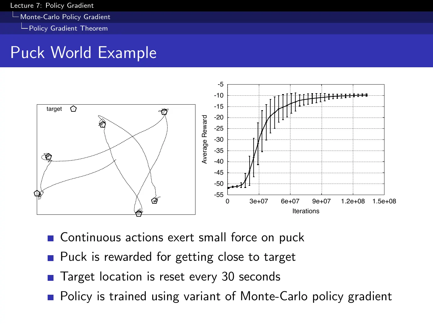
Low-friction puck, continuous forces, target relocated every 30 seconds. Two things to take from the plot, and the second is the reason the lecture continues:

The curve is smooth. No chattering, no collapses — the visual contrast with value-based learning curves is the point.
The x-axis runs to roughly $10^8$ iterations. REINFORCE solves this, slowly. Estimating a gradient from complete returns is extremely high variance.

The slide's own figure text records the other cost from p.5: 4 runs out of 100 converged to substantially suboptimal local minima. The local-optimum disadvantage is not hypothetical.

7 · Actor-critic

p.23–25 · Reducing Variance Using a Critic ⏱ 52:52

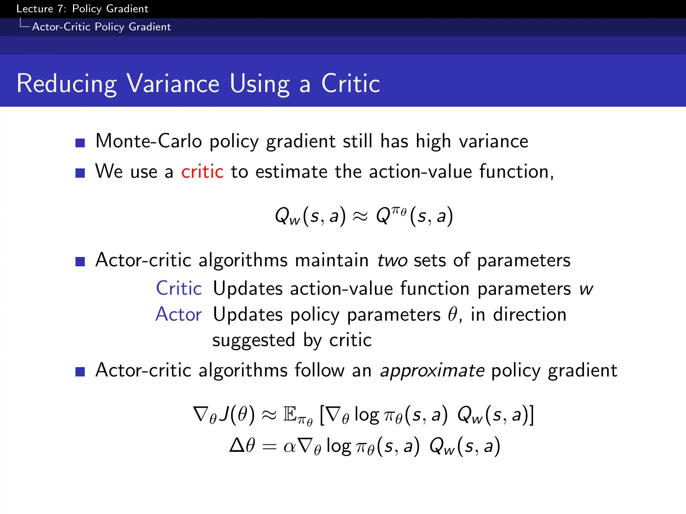
Replace the noisy return with an explicit estimate $Q_w(s,a)\approx Q^{\pi_\theta}(s,a)$ . Two parameter sets now: the actor $\theta$ picks actions, the critic $w$ judges them without ever acting.

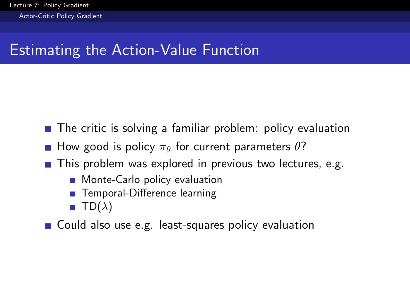
The critic's job is policy evaluation — the exact problem of L4 and L6. Any evaluation algorithm slots in: MC, TD(0), TD( $\lambda$ ), LSTD. Note what is not being estimated: the critic estimates $Q^{\pi_\theta}$ for the current policy, not $q_*$ . There is no max anywhere.

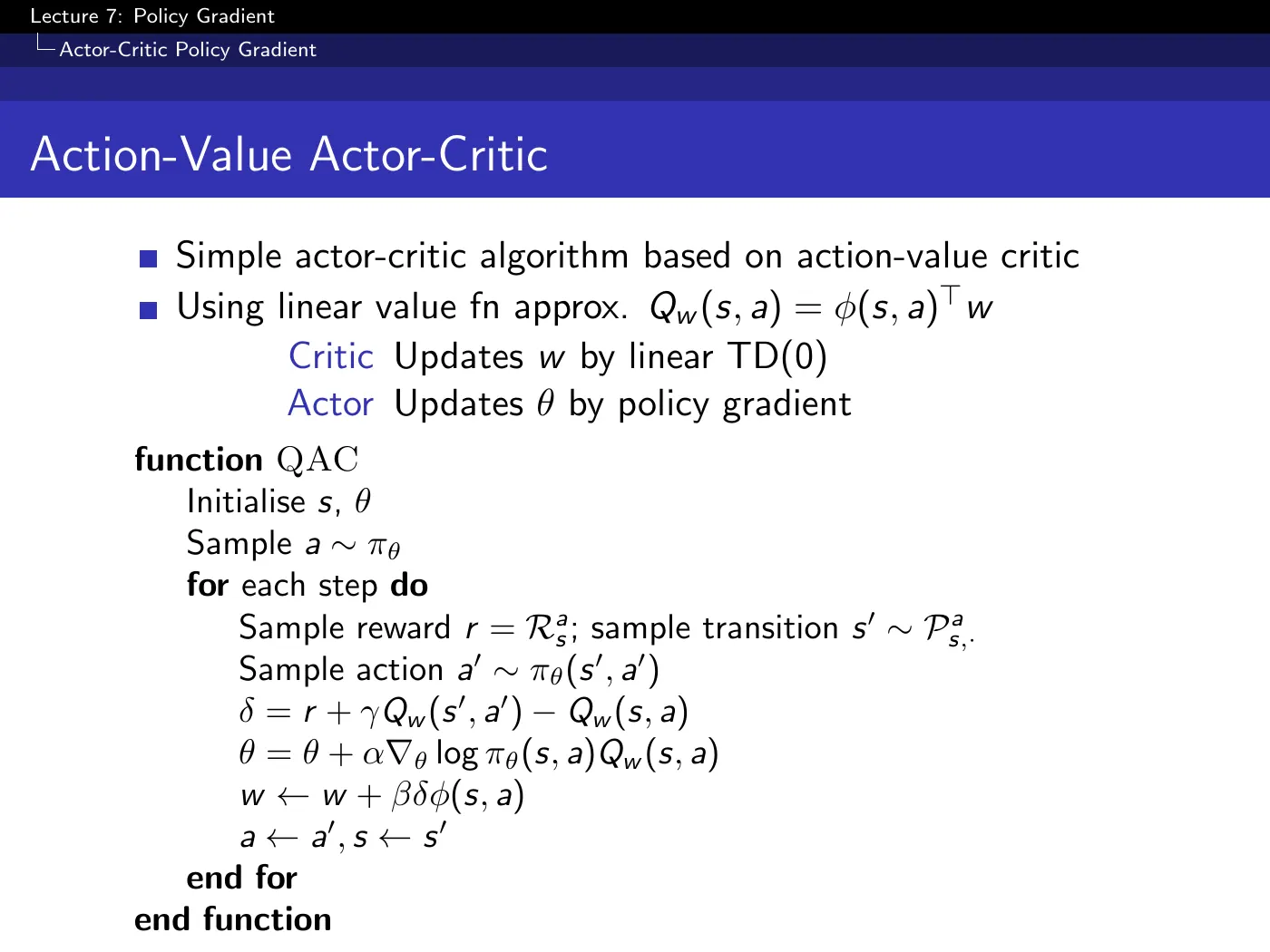
QAC is fully online — every step updates both critic and actor. Compare against REINFORCE, which needed a complete episode.

Is actor-critic just generalized policy iteration again?

Yes, with the improvement step swapped. Evaluate the current policy with the critic, then improve it — except improvement is now a small gradient step instead of a greedy jump. Same GPI skeleton as L3 and L5, with the aggressive operator replaced by a gentle one.
That substitution is exactly what buys the smooth curve on p.22 and costs the sample efficiency.

Is greedy action selection recoverable as a special case?

In some tabular softmax and natural-gradient formulations, making the update increasingly aggressive approaches a greedy policy-improvement step. That is a useful bridge between the two families, but not a universal identity: parameterization, regularization, action support, and step size all matter. The safe intuition is simply that policy gradient permits gradual improvement, while greedy improvement replaces the action choice immediately.

L3 proved convergence to a global optimum by contraction. What survives here?

The lecture's practical message is comparative: smooth policy updates often behave better than repeated greedy replacements. That is not a Bellman-contraction proof. With a general parameterized policy, the objective is non-convex and local stationary points remain possible. Stronger global-convergence results require specific tabular parameterizations, sampling assumptions, and step-size conditions; do not transfer them automatically to neural policies.

8 · Removing the bias, reducing the variance

p.26–28 · Compatible Function Approximation ⏱ 1:23:27

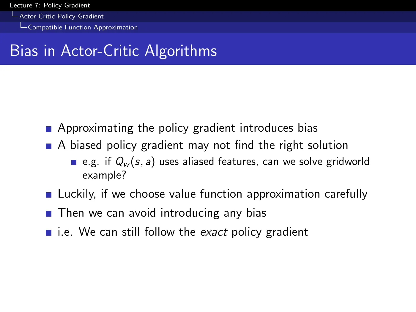
The question nobody thinks to ask. On p.23 the true $Q^{\pi_\theta}$ was quietly swapped for an approximation $Q_w$ , and everyone carried on. Why is the resulting direction still a gradient of anything? In general it is not — approximating the critic biases the policy gradient, and a biased gradient can converge to the wrong policy.

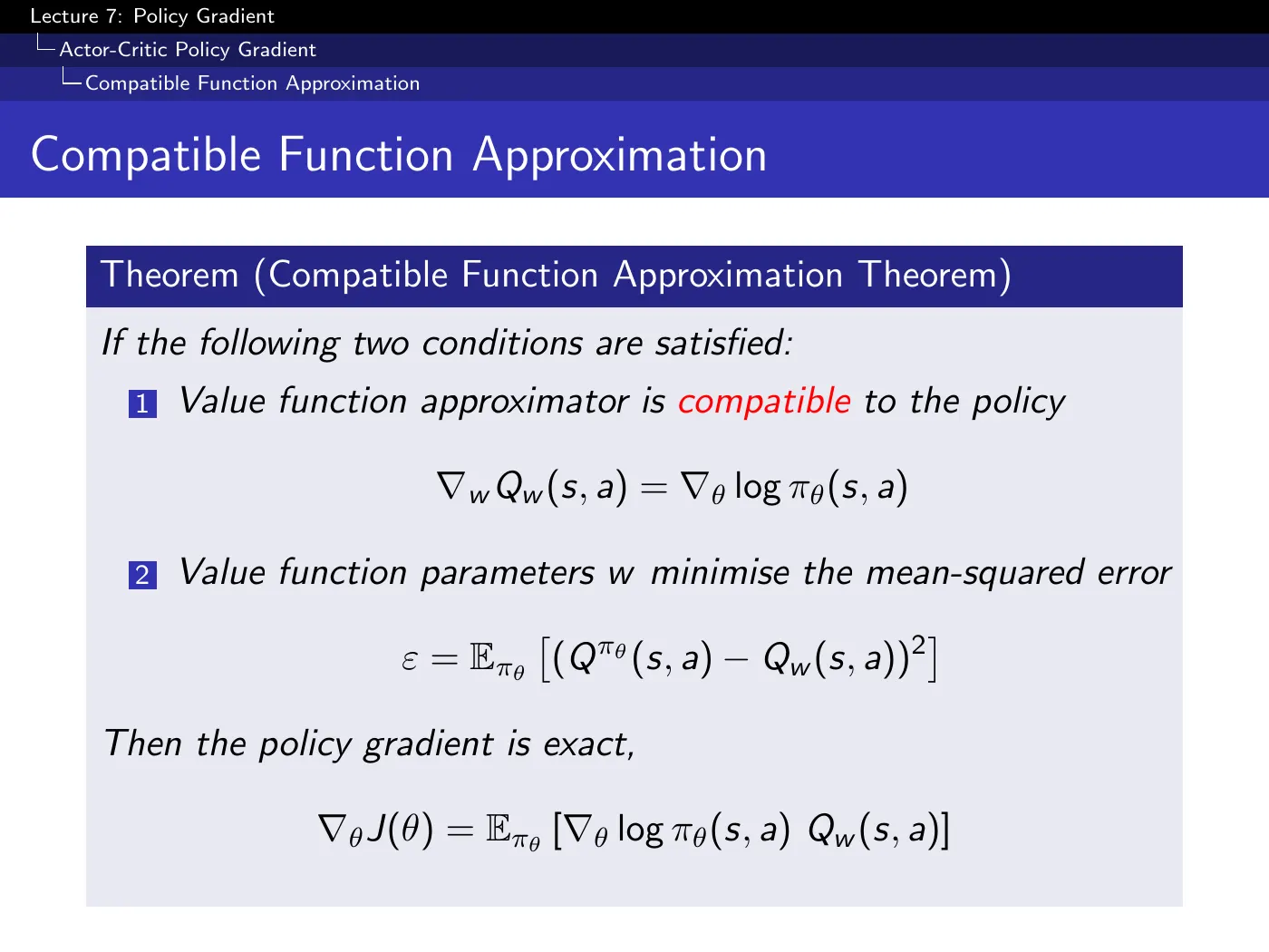
Two conditions make the bias exactly zero:

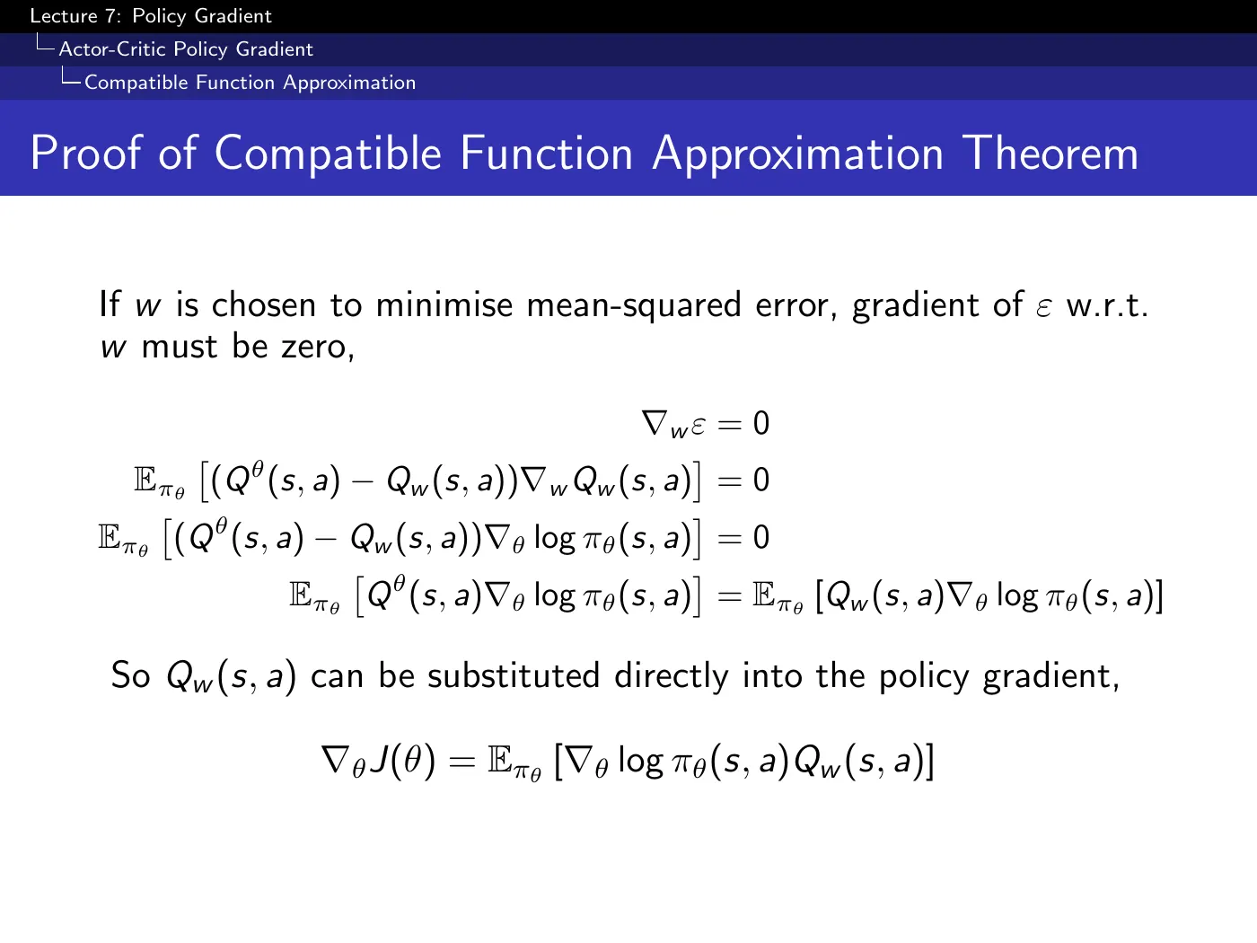
\text{(1)}\quad\nabla_w Q_w(s,a)=\nabla_\theta\log\pi_\theta(s,a) \qquad\qquad \text{(2)}\quad w \text{ minimizes } \varepsilon=\mathbb{E}_{\pi_\theta}\big[(Q^{\pi_\theta}(s,a)-Q_w(s,a))^2\big]

The proof is four lines and worth following once. Condition (2) gives $\nabla_w\varepsilon=0$ ; substituting condition (1) into it produces an expectation that says the error between the true and approximate gradients is itself zero. So $Q_w$ can be dropped into the policy gradient unchanged.

What condition (1) really demands

Integrating it says the critic must be linear in the score function: $Q_w(s,a)=\nabla_\theta\log\pi_\theta(s,a)^\top w$ . Your critic's features are forced to be the policy's score — you do not get to choose them.
That is a severe restriction, and it is why compatible function approximation reads as a theoretical reassurance ("an unbiased actor-critic exists") more than as a recipe anyone follows. The lecture flags the theorem and moves on without applying it.

p.29 · Reducing Variance Using a Baseline ⏱ 1:06:38

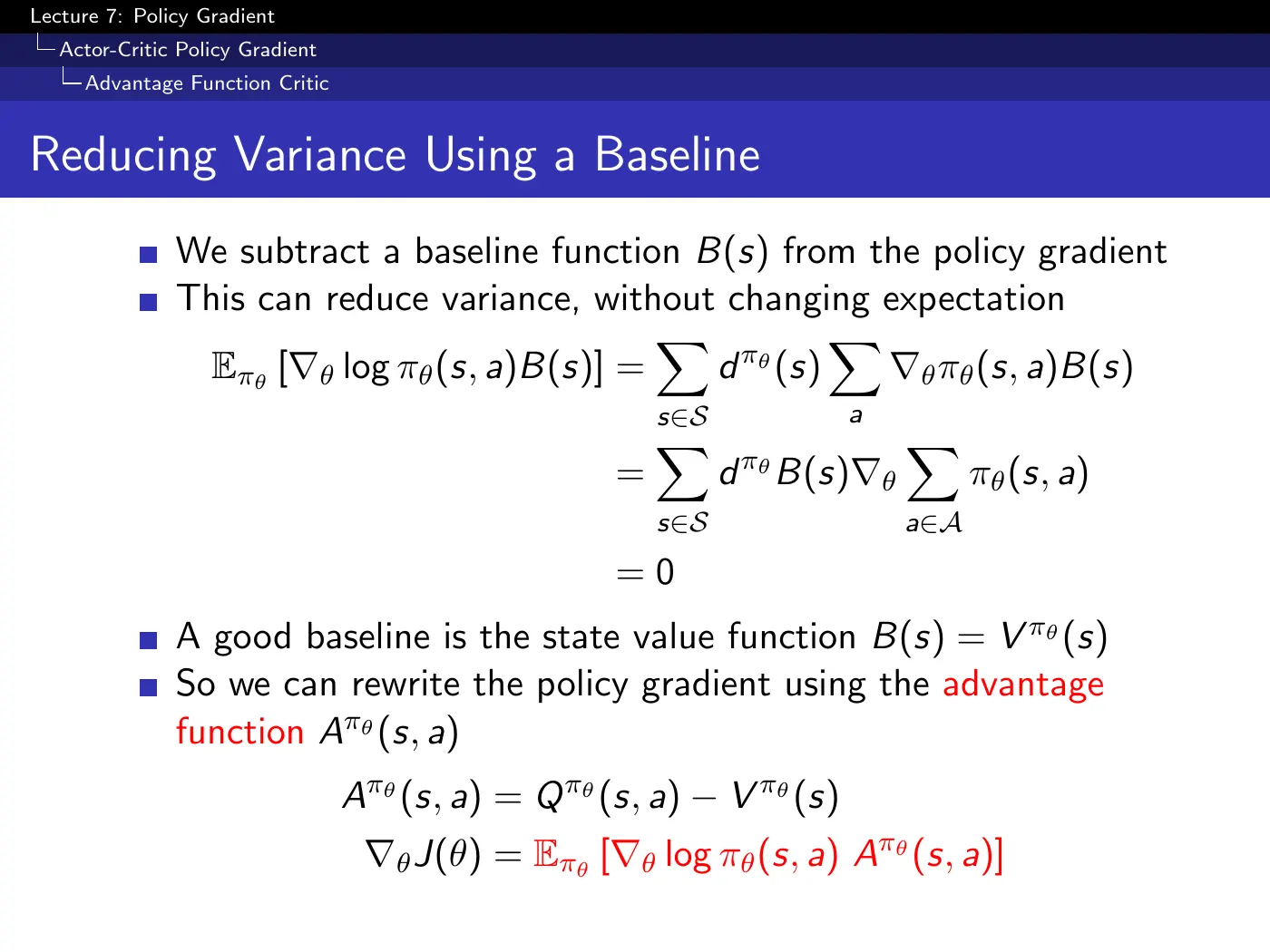
\mathbb{E}_{\pi_\theta}[\nabla_\theta\log\pi_\theta(s,a)B(s)]=\sum_s d^{\pi_\theta}(s)B(s)\nabla_\theta\underbrace{\sum_a\pi_\theta(s,a)}_{=1}=0

Subtract any function of state and the expectation is unchanged, because the policy sums to one and the gradient of a constant is zero.

Why you would want to — the part the slide omits

Suppose one action returns $1{,}000{,}000$ and another returns $999{,}000$ . Both are large and positive, so both push the policy toward taking them, differing only in strength. The update is dominated by an offset that carries no information about which action was better.
A baseline recenters the scale so that better-than-usual is positive and worse-than-usual is negative. Only then does the update mean "do more of this, less of that" rather than "do more of everything, at various speeds."

The constraint is that $B$ depends on state only. If it depended on the action, it would not factor out of $\sum_a$ and the expectation would change — that is the entire content of the derivation.

The natural choice is $B(s)=V^{\pi_\theta}(s)$ , which turns $Q$ into the advantage function:

A^{\pi_\theta}(s,a)=Q^{\pi_\theta}(s,a)-V^{\pi_\theta}(s),\qquad \nabla_\theta J(\theta)=\mathbb{E}_{\pi_\theta}\big[\nabla_\theta\log\pi_\theta(s,a)A^{\pi_\theta}(s,a)\big]

"How much better than usual is this action" — the same phrase the score functions on p.17–18 produced from the other side. The two halves of the update now match in form.

p.30–31 · Estimating the Advantage Function ⏱ 1:11:57

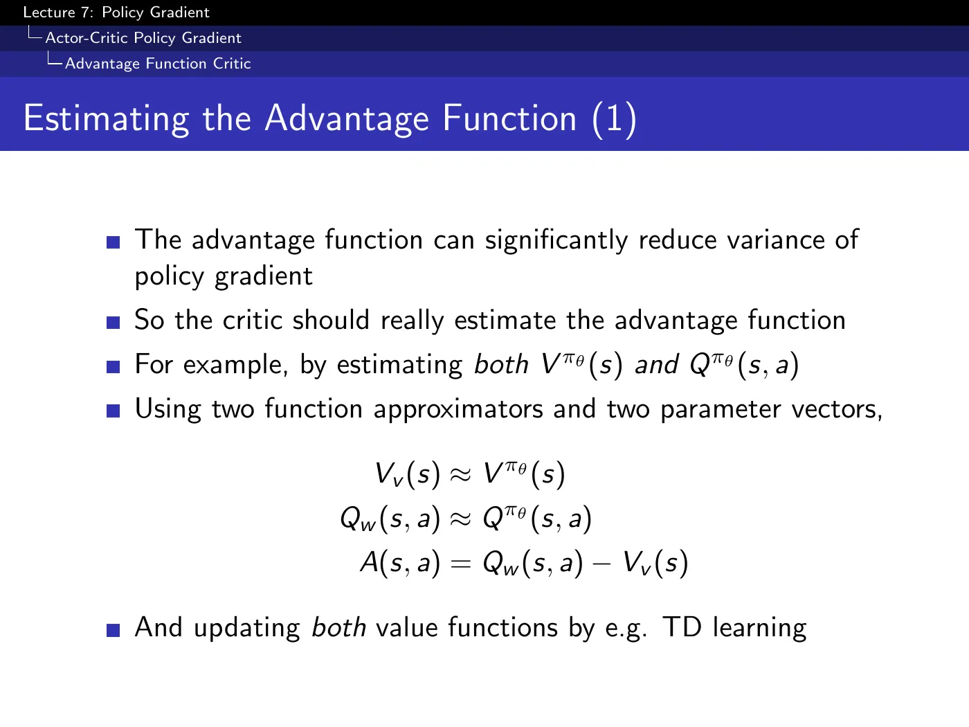
The direct route needs two approximators and two parameter vectors, $V_v$ and $Q_w$ . It works and it is clumsy.

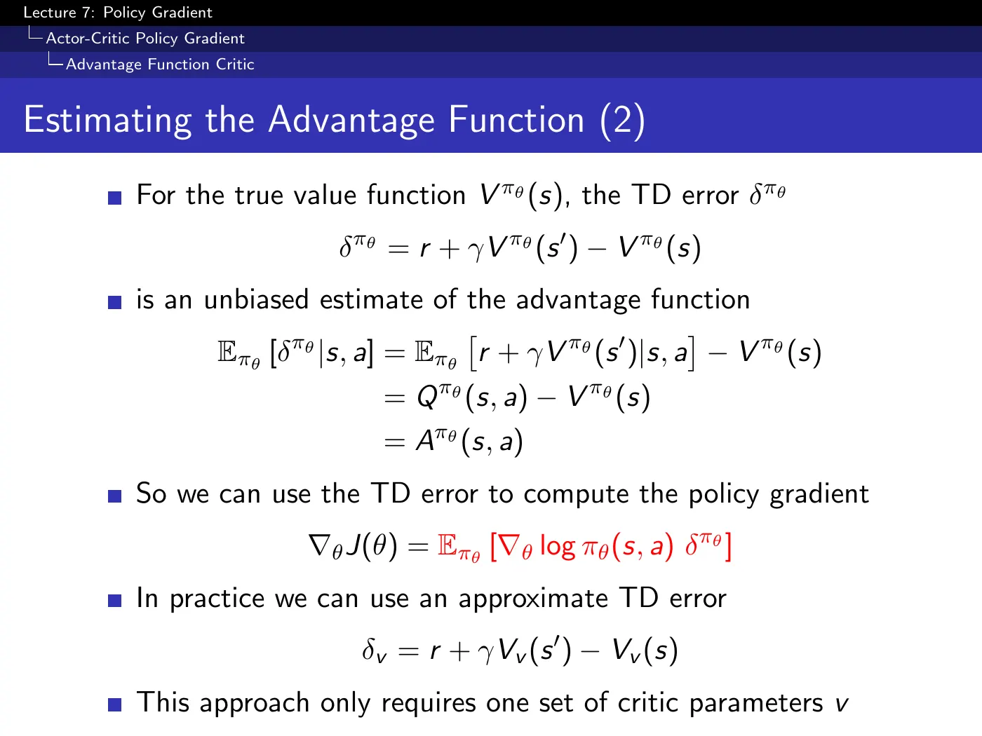
The better route, in three lines:

\mathbb{E}_{\pi_\theta}[\delta^{\pi_\theta}\mid s,a]=\underbrace{\mathbb{E}_{\pi_\theta}[r+\gamma V^{\pi_\theta}(s')\mid s,a]}_{=\;Q^{\pi_\theta}(s,a)}-V^{\pi_\theta}(s)=A^{\pi_\theta}(s,a)

The pivot is that $\mathbb{E}[r+\gamma V^\pi(s')\mid s,a]$ is $Q^\pi(s,a)$ — half a Bellman unroll, and the same "use an identity to justify a sampled quantity" move as p.19. The payoff is large: the TD error is an unbiased sample of the advantage, so the critic needs to estimate only $V$ , with one parameter vector and no actions in it.

"Unbiased" is a claim about the true

V^{\pi_\theta}

, not about your critic

The derivation uses the exact $V^{\pi_\theta}$ . The last bullet then says that in practice you use $\delta_v=r+\gamma V_v(s')-V_v(s)$ — and with an approximate $V_v$ , $\delta_v$ is biased again.
The slide makes the swap in one line without flagging that it gives back exactly the guarantee the previous three slides were about. In practice this is accepted; just do not carry "the TD error is unbiased" forward as though it applied to the algorithm you actually run.

p.32–34 · Different Time-Scales, and Traces ⏱ 1:17:19

This slide reuses

\theta

for the critic's parameters

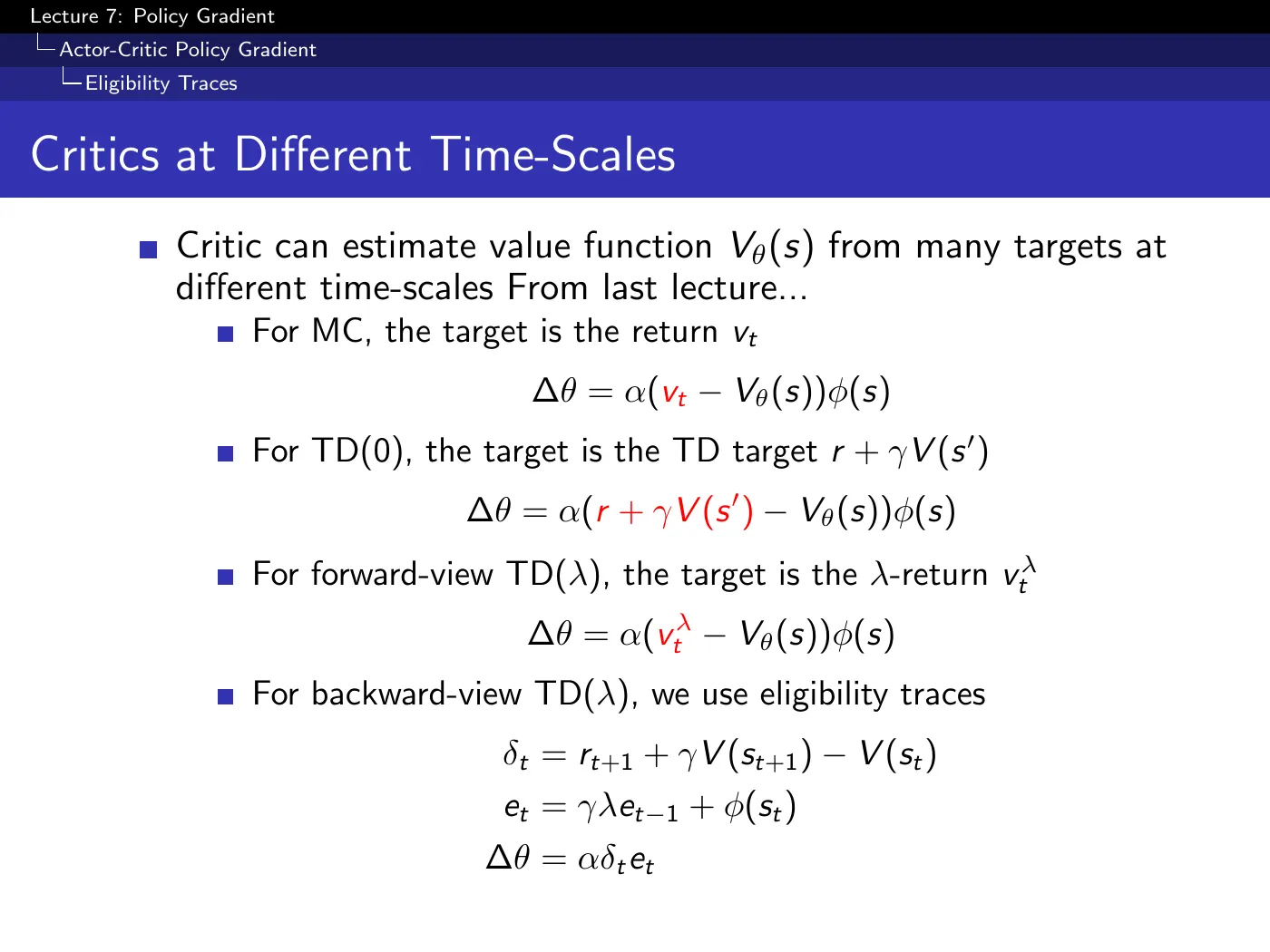
The critic here is written $V_\theta(s)$ with updates $\Delta\theta$ — but $\theta$ is the actor's parameter vector everywhere else in the deck, and p.30–31 correctly call the critic's parameters $v$ . Silver flags the slip verbally mid-lecture.
Read every $\theta$ on this slide as $v$ . The content is just L6's menu of critic targets, unchanged.

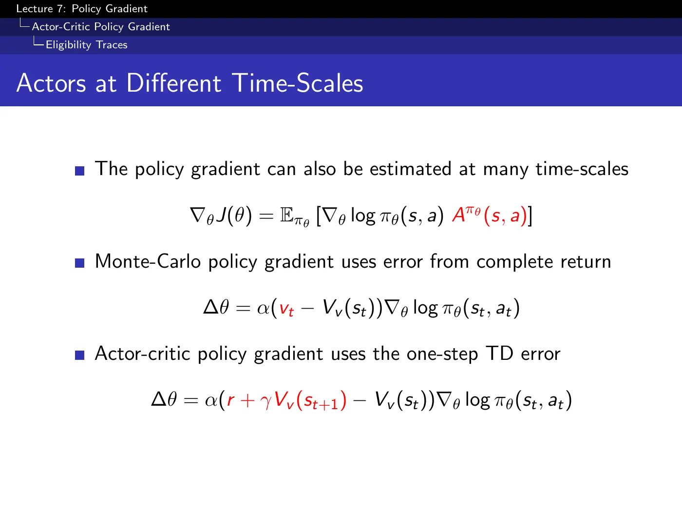
The critic's time-scale and the actor's time-scale are independent choices. You can give the critic TD( $\lambda$ ) and still update the actor from a one-step error. This slide asks the separate question: can the actor also mix time-scales?

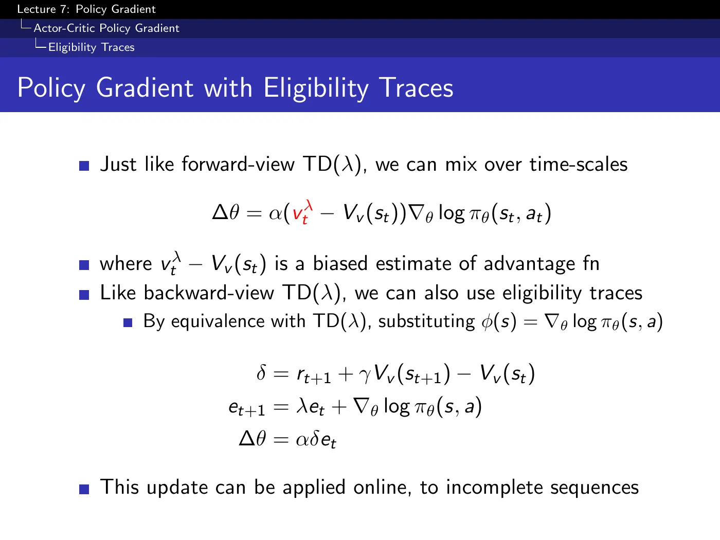
\delta=r_{t+1}+\gamma V_v(s_{t+1})-V_v(s_t),\qquad e_{t+1}=\lambda e_t+\nabla_\theta\log\pi_\theta(s,a),\qquad \Delta\theta=\alpha\,\delta\,e_t

The transfer rule is mechanical — search and replace

Everywhere value-based TD( $\lambda$ ) used $\nabla_\theta\hat v$ or the feature vector $\phi(s)$ , substitute the score $\nabla_\theta\log\pi_\theta(s,a)$ . The same forward/backward-view construction carries across after this substitution, but the objective, discount, and occupancy-measure conventions still have to match.
The trace now accumulates scores, so it remembers which directions in policy-parameter space have recently been responsible for the actions taken — recency and frequency, exactly as before, one level up. → Forward and Backward Views of TD Lambda

The payoff is the last bullet: unlike REINFORCE, this runs online and on incomplete sequences.

Do not implement the trace from this slide without fixing the convention

p.32 gives the critic trace as $e_t=\gamma\lambda e_{t-1}+\phi(s_t)$ , while p.34 gives the actor trace without $\gamma$ . Under the usual discounted episodic backward view, the actor trace also decays by $\gamma\lambda^\theta$ , and actor and critic may use different trace rates and step sizes. Some formulations additionally carry a discount accumulator for the start-state objective. The correct code therefore depends on whether the objective is discounted episodic or continuing average reward; the slide mixes notation and does not specify enough to copy verbatim.

9 · What the deck does not have

Deterministic policy gradient ⏱ 1:26:32

There is no slide for this section. It is taught in the video and absent from this PDF. Recorded here because the argument is short, load-bearing, and became the basis of DDPG.

The problem it solves is genuinely surprising:

A stochastic policy gets harder to estimate as it gets better

Policy gradient estimates the gradient by sampling the policy's own noise. As a Gaussian policy narrows — $\sigma\to 0$ , which is exactly what learning is supposed to do — the variance of the gradient estimate blows up toward infinity.
Success makes estimation worse. That is the opposite of what you want from an algorithm, and it is a structural property of every stochastic policy gradient method above.

The fix is to stop narrowing a noisy policy toward determinism and start deterministic, taking the limiting case of the policy gradient theorem directly. What comes out is a chain rule:

\nabla_\theta J(\theta)=\mathbb{E}\big[\nabla_\theta\mu_\theta(s)\,\nabla_a Q^w(s,a)\big|_{a=\mu_\theta(s)}\big]

Read it right to left and it is obvious in hindsight: the critic already knows which way to move the action. $\nabla_a Q$ says "push the torque a little higher and you get more reward." $\nabla_\theta\mu_\theta$ says how to change the parameters so the policy outputs that. No score function, no sampling your own noise.

Two conditions on it: continuous action spaces only (there is no $\nabla_a$ over discrete actions), and it requires a $Q$ -critic rather than a $V$ -critic. Reported in the lecture as working considerably better than stochastic policy gradient at high action dimensionality.

Restored from the spoken derivation, since no slide exists — verify the exact statement against Silver et al., Deterministic Policy Gradient Algorithms, ICML 2014.

p.41 · Summary of Policy Gradient Algorithms ⏱ 1:30:21

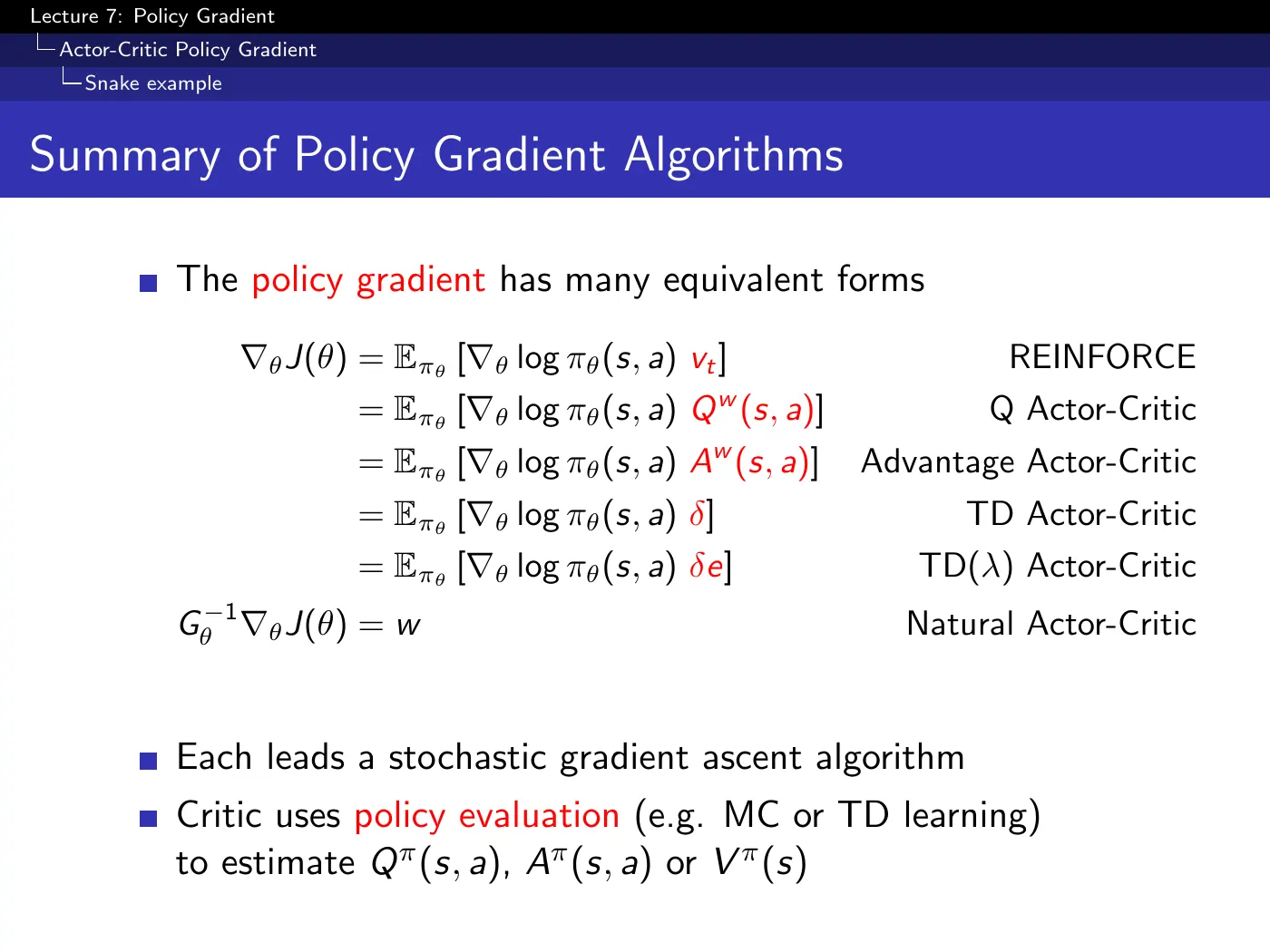
The most useful slide in the lecture, and the one to reconstruct from memory. Every row is the same equation with a different second factor, and the critic under each is free to be MC, TD, TD( $\lambda$ ), or least squares.

The video's version of this slide has a different last row

This PDF ends with Natural Actor-Critic, matching p.35–37 which the video skips. The video's summary instead lists Deterministic Actor-Critic, matching the section above which this PDF lacks.
When you reconstruct the table, know that it has six rows in one version and six in the other — but not the same six.

Study checklist

Close the note and answer these in your own words. Reopen only the section linked after the question.

What changes when the policy, rather than the value function, is parameterized directly? → 1 · Why parameterize the policy
Give the two distinct reasons a stochastic policy can be necessary. → 2 · When you actually need randomness
Why does state aliasing break the deterministic-policy result from a fully observed MDP? → p.7–9 · Aliased Gridworld ⏱ 15:25
Why must the objective and its state-distribution convention be stated together? → 3 · What best even means
What does the likelihood-ratio identity convert into something that can be sampled? → 5 · The score function
State the policy-gradient theorem and explain the roles of its two factors. → 6 · The policy gradient theorem
How does REINFORCE estimate $Q^{\pi_\theta}$ , and why is its variance high? → p.21–22 · REINFORCE and Puck World ⏱ 48:13
What does the critic estimate, and how does actor-critic relate to GPI? → 7 · Actor-critic
Why can a state-only baseline reduce variance without changing the expected gradient? → p.29 · Reducing Variance Using a Baseline ⏱ 1:06:38
When is the TD error an unbiased sample of advantage, and what changes with an approximate critic? → p.30–31 · Estimating the Advantage Function ⏱ 1:11:57
What must be checked before implementing the eligibility-trace formula from p.34? → p.32–34 · Different Time-Scales, and Traces ⏱ 1:17:19
Why does deterministic policy gradient require continuous actions and a differentiable $Q$ -critic? → Deterministic policy gradient ⏱ 1:26:32

Gaps to close on your own

Slides p.35–37 are skipped in the lecture — natural policy gradient

The video jumps from the eligibility-trace slide straight to the summary, explicitly deferring this block to the notes.

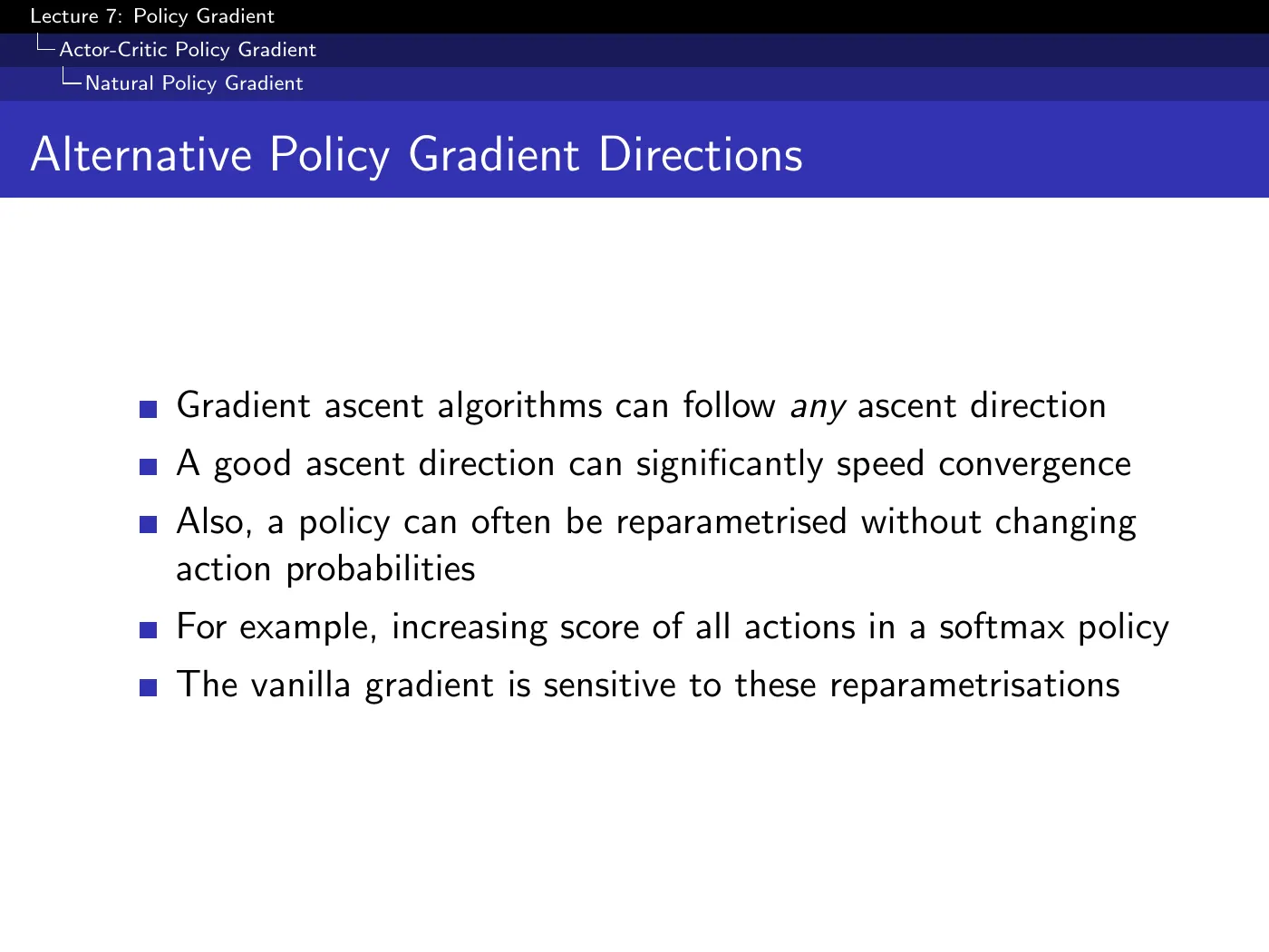
The motivation is the one thing you can read off without the lecture: a policy can be reparameterized without changing any action probabilities — for instance, adding a constant to every score in a softmax. The vanilla gradient is sensitive to such reparameterizations, so it can point in a direction that is an artifact of how you happened to write the policy down.

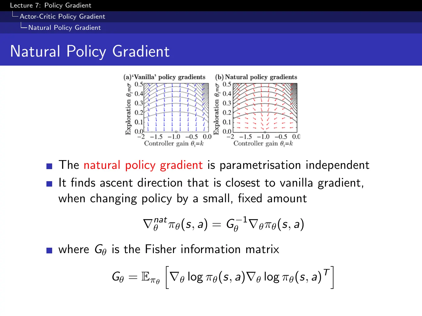
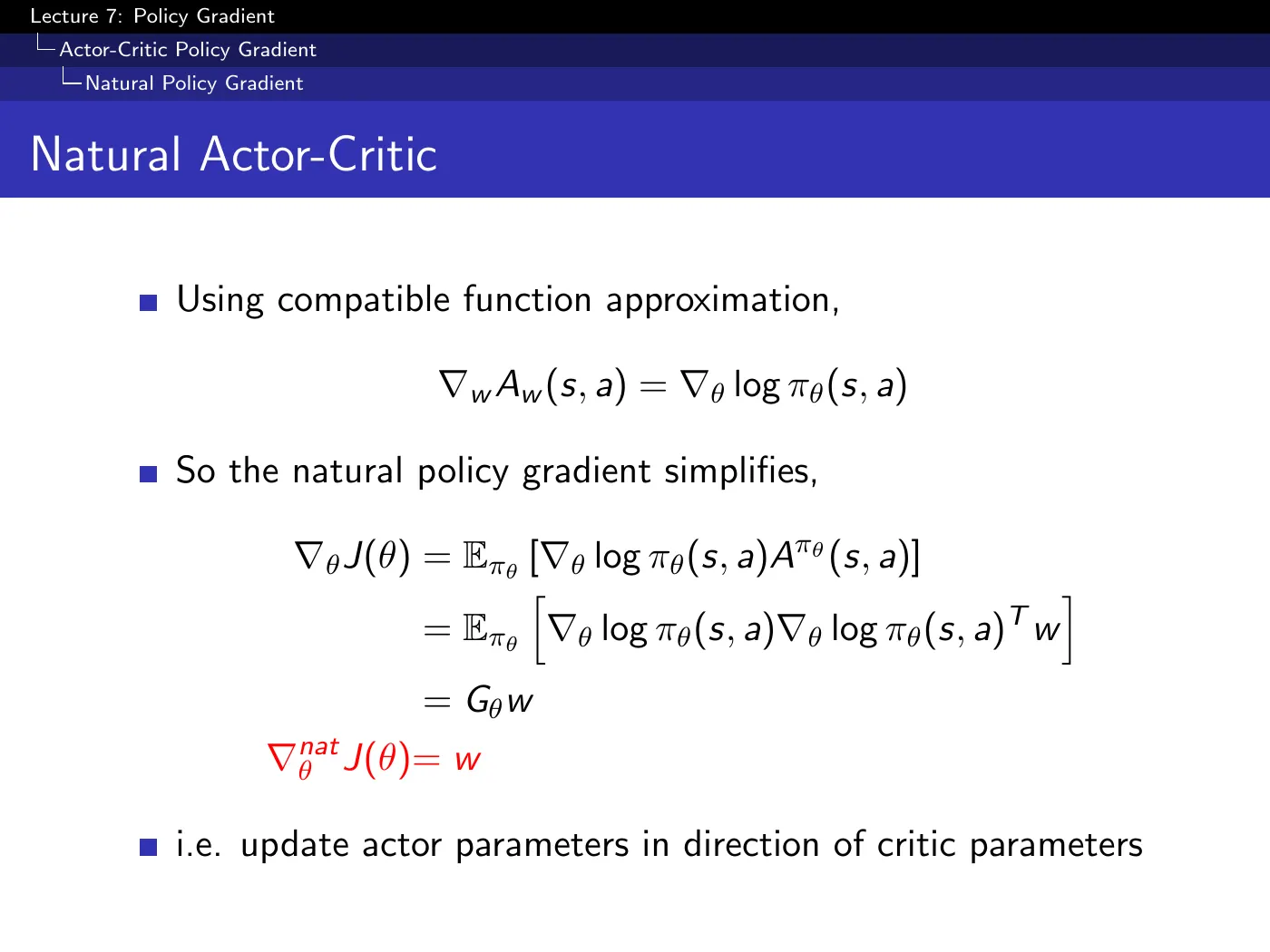
The natural gradient $\nabla^{nat}_\theta=G_\theta^{-1}\nabla_\theta$ , with $G_\theta$ the Fisher information matrix, is parameterization-independent. p.37 is the punchline worth understanding: under compatible function approximation the natural policy gradient simplifies to $w$ itself — update the actor in the direction of the critic parameters. The snake demo on p.38–40 illustrates it and is also skipped. This direction is what TRPO steps along in practice, computed with conjugate gradient instead of an explicit inverse → Lee 2020 notes §2.

The deterministic policy gradient has no slide here. Restored above from the spoken derivation. Sutton & Barto does not derive it either — DPG appears only as a citation in the Chapter 13 bibliographic notes. So this one has to come from Silver et al., Deterministic Policy Gradient Algorithms, ICML 2014. Worth the trip: it is the direct ancestor of DDPG, the algorithm you will actually meet in robot-control papers → RL-based Humanoid Locomotion.
Global optimum for tabular softmax is asserted in the lecture, but Silver misspoke mid-sentence ("local" for "global"). Not settled by Sutton & Barto — the book discusses global optima only for linear value function approximation, never for softmax policy gradient. This is a more recent result than the textbook; look to the global-convergence literature on softmax policy gradient rather than to S&B.
Compatible function approximation in practice. The theorem is stated and the restriction it imposes is severe. Whether anyone actually uses it, and what modern actor-critic methods do about critic bias instead, is not addressed here — nor by Sutton & Barto, who do not cover the theorem at all.
Where the score function comes from statistically. It is introduced as an algebraic identity, but it is the same score function as in maximum likelihood estimation and Fisher information (which reappears on the skipped p.36). Worth reading once from the statistics side.

Language notes

Phrasings worth stealing for your own technical writing and talks:

Expression	Use
how much more than usual	naming a quantity measured against a baseline
get the best of both worlds	a method inheriting the advantages of two extremes
extract the most juice from	maximize what you get out of a fixed resource
break open the trajectory	use intermediate structure instead of one summary number
until your grad students collapse of exhaustion	conceding an approach does not scale, wryly
it should be the first question that you ask	flagging an obvious objection everyone skips
we substituted in something and hoped	naming an unjustified step before justifying it
a big soup of possible things to follow	admitting a design space is wide and underdetermined
this is really just a rewrite — we haven't changed anything	signalling algebraic restatement, not a new claim
an unfortunate property of	a structural drawback that is nobody's fault