Lecture 8 · Integrating Learning and Planning

Slides: David Silver - RL Course (UCL 2015) · Previous: Lecture 7 · Policy Gradient · Next: Lecture 9 · Exploration and Exploitation

First pass: read The one idea and the slide-group headings. Use the prose when an equation, condition, or figure needs explanation; leave Gaps to close for review.

The one idea

Three lectures, three things to learn from experience:

What you learn directly from experience	Lecture
a value function	L4–L6
a policy	L7
a model of the environment	L8

Learning a model does not replace the learner. It multiplies the transitions available to it: most sample-based methods from L4 through L7 can consume a simulated tuple through the same update interface used for a real tuple. Whether the resulting update is valid still depends on model accuracy and on-policy/off-policy assumptions.

The model turns finite experience into unlimited simulated transitions

A real robot produces experience slowly and expensively. A model of that robot produces transitions as fast as you can compute. These are not new independent facts about the real world — every simulation inherits the model's errors — but they let the agent spend compute to propagate and test what its real experience has already taught it.
This is the entire economic argument for model-based RL, and every algorithm in the lecture is a way of spending the second budget.

Sample-based planning — the model's job is to produce samples, not probabilities

Dynamic programming used $\mathcal{P}^a_{ss'}$ to integrate over every outcome. Sample-based planning does not enumerate those probabilities; it asks a generative model for transitions. The probabilities are still present implicitly in the sampler. This often saves work because common outcomes are sampled often and very unlikely outcomes rarely.
The consequence is that this lecture contains almost no new mathematics. Once experience is being generated, you reach for Monte-Carlo control, Sarsa, or Q-learning unchanged.

The three architectures, which is the spine of the lecture:

	Learn from real experience	Learn from simulated experience
Model-free RL (L4–L7)	value / policy	—
Model-based RL	model only	value / policy
Dyna	value / policy and model	value / policy

1 · Why bother learning a model
2 · What a model is, and how to learn one
3 · Planning by sampling
4 · When the model is wrong
5 · Dyna
6 · Forward search
7 · Monte-Carlo tree search
8 · TD search and Dyna-2
Study checklist
Gaps to close on your own
Language notes

1 · Why bother learning a model

p.4–8 · Model-Based and Model-Free RL ⏱ 6:18

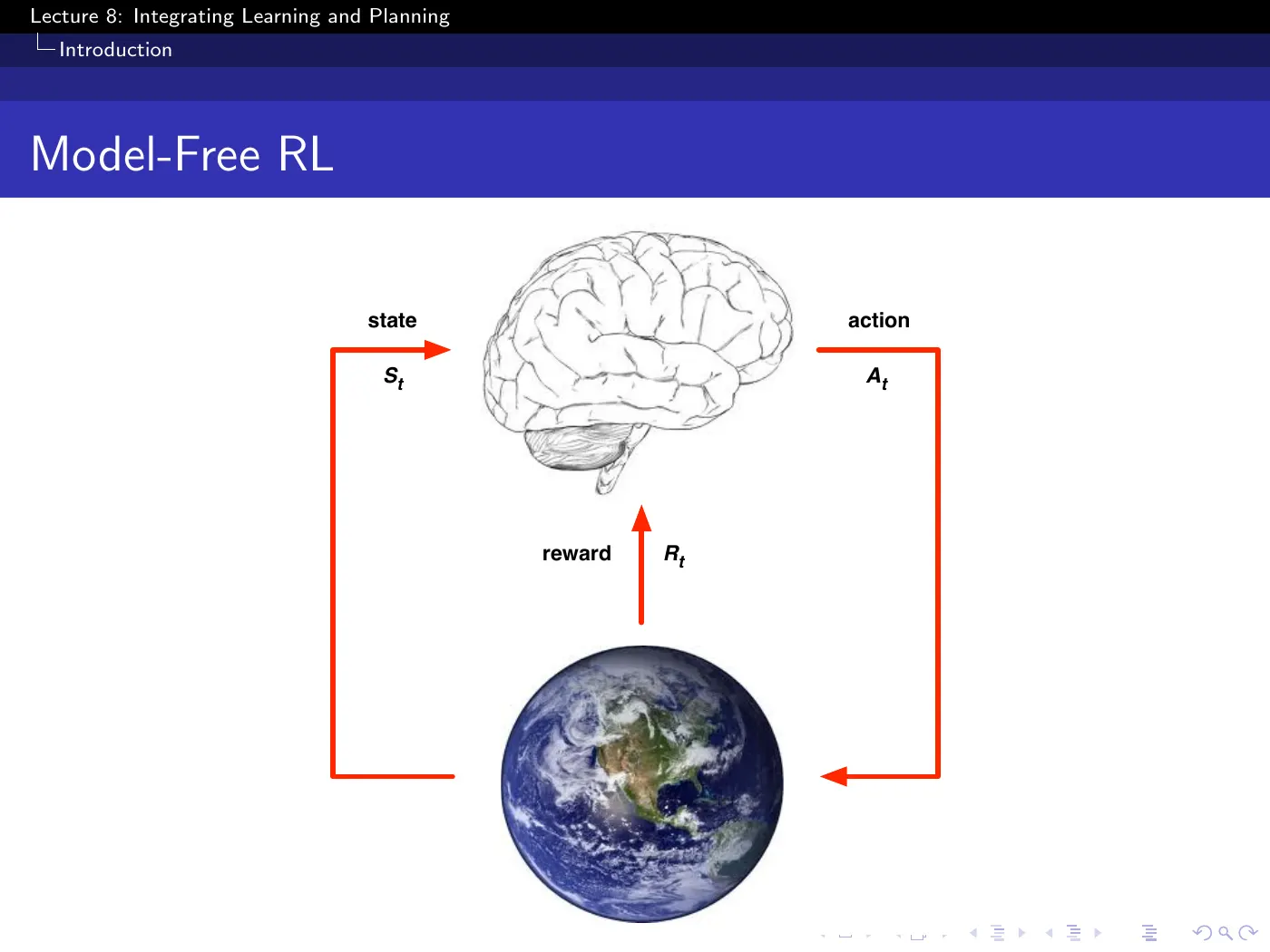
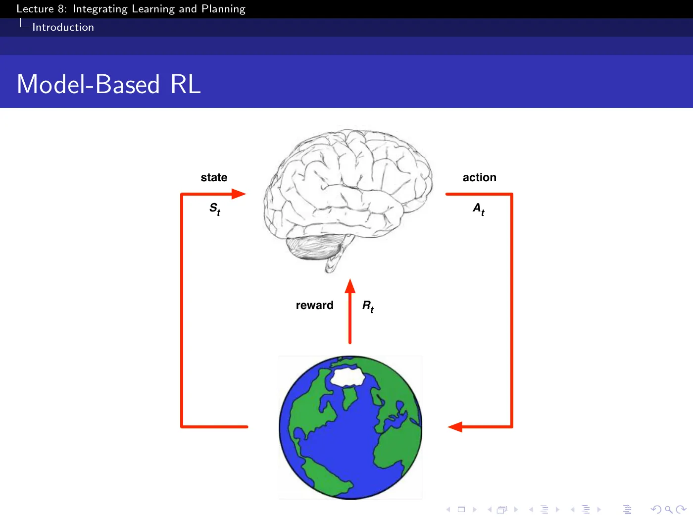
Lecture 8 Integrating Learning and Planning, slide 7

Lecture 8 Integrating Learning and Planning, slide 8

These two slides are the whole lecture in a picture, and the difference between them is easy to skim past: the environment has been replaced by the agent's cartoon of the environment. The loop is otherwise identical — observe state, take action, receive reward — except none of it happens.

That is the first time in this course an agent can improve without interacting with the world at all. Everything from L4 to L7 required fresh experience to make progress; here, thinking is a form of progress.

p.10 · The Model-Based RL Cycle ⏱ 9:19

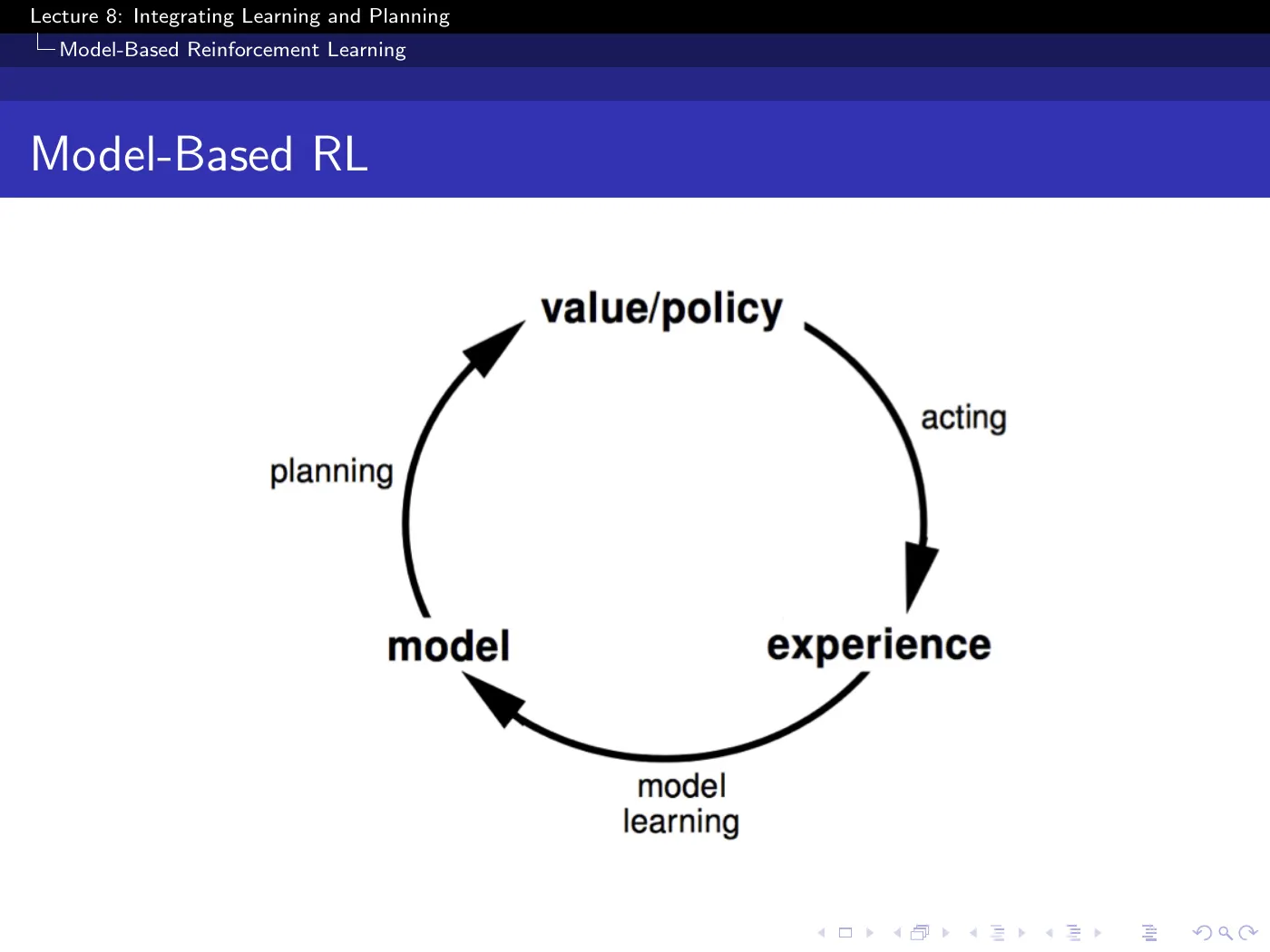
Lecture 8 Integrating Learning and Planning, slide 10

Experience → model → plan → value/policy → act → more experience. Read the two inserted steps as what they literally are: learn an MDP, then solve it.

This answers a limitation stated five lectures ago

L3 developed value iteration and policy iteration and then set them aside for RL, because they require being told $\langle\mathcal{P},\mathcal{R}\rangle$ . L8's reply is simply: then learn $\langle\mathcal{P},\mathcal{R}\rangle$ first.
Every planning algorithm from L3 becomes available the moment you have a model. The "planning" box in this diagram is L3 in its entirety.

p.11 · Advantages of Model-Based RL ⏱ 11:35

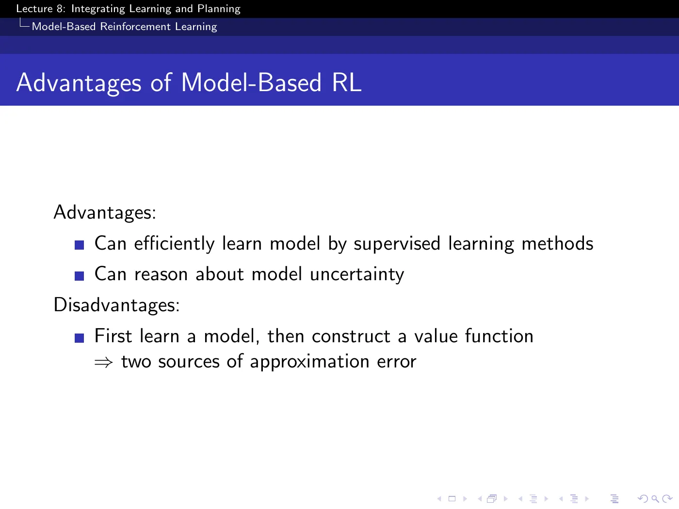
Lecture 8 Integrating Learning and Planning, slide 11

The slide lists advantages flatly. The argument that actually carries them is Silver's chess example, which appears on no slide:

Why a model can be the compact object

Chess has on the order of $10^{48}$ states and an extremely sharp value function — move one piece one square and a won position becomes a lost one. Learning $v$ or $\pi$ directly across that landscape is very hard.
The model is just the rules of the game: move this pawn two squares and you are in that position. Trivial to represent, trivial to learn. So the sensible route to a good value estimate is to plan with the easy object rather than to learn the hard one.
This is the general case for planning: there exist MDPs where it is very hard to say who is ahead without looking ahead.

Isn't learning the reward function the same problem as learning the value function?

No, and the gap between them is enormous. In chess the reward function is $0$ at every non-terminal step and $\pm 1$ at the end. Learning it means learning to answer "is this checkmate?" — essentially a classification of whether the king has a legal move.
Learning the value function means answering "from this complicated middlegame position, what is the probability White wins?" — which requires understanding the whole game.
Reward is a local, immediate, one-step fact. Value is a global, long-horizon one. Model-based RL exploits exactly that asymmetry: learn the easy local facts, and recover the hard global ones by look-ahead.

The disadvantage is real and worth stating precisely: you now have two sources of approximation error in series. The model is approximate, and the value function built from it is approximate, and those errors compound. Model-free RL has only the second.

2 · What a model is, and how to learn one

p.12 · What is a Model? ⏱ 15:23

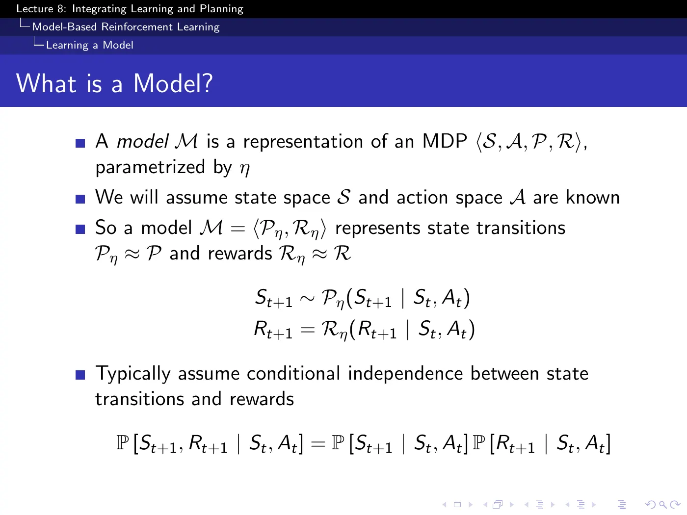
Lecture 8 Integrating Learning and Planning, slide 12

\mathcal{M}_\eta=\langle\mathcal{P}_\eta,\mathcal{R}_\eta\rangle,\qquad S_{t+1}\sim\mathcal{P}_\eta(\cdot\mid S_t,A_t),\qquad R_{t+1}\sim\mathcal{R}_\eta(\cdot\mid S_t,A_t).

"Model" is one of the most overloaded words in science; here it means precisely one thing — the agent's estimate of the MDP it is living in.

Two simplifications are being made quietly:

$\mathcal{S}$ and $\mathcal{A}$ are assumed known. Only $\mathcal{P}$ and $\mathcal{R}$ are learned. Learning the state space itself is possible and is a much harder problem.
Transitions and rewards are assumed conditionally independent, so they can be learned separately. Convenient, not necessary.

If you get to choose the features, why assume the state space is given?

Because it keeps the lecture tractable — but the assumption is doing real work. The raw inputs you are handed may be useless for predicting dynamics even if they are fine for other purposes, and in that case the first thing you want is a better state representation.
Silver concedes this outright: learning your own features is typically a very good idea, and learning the state or action space is a legitimate but more complicated version of the problem. Modern model-based deep RL is largely about exactly this.

p.13 · Model Learning ⏱ 22:14

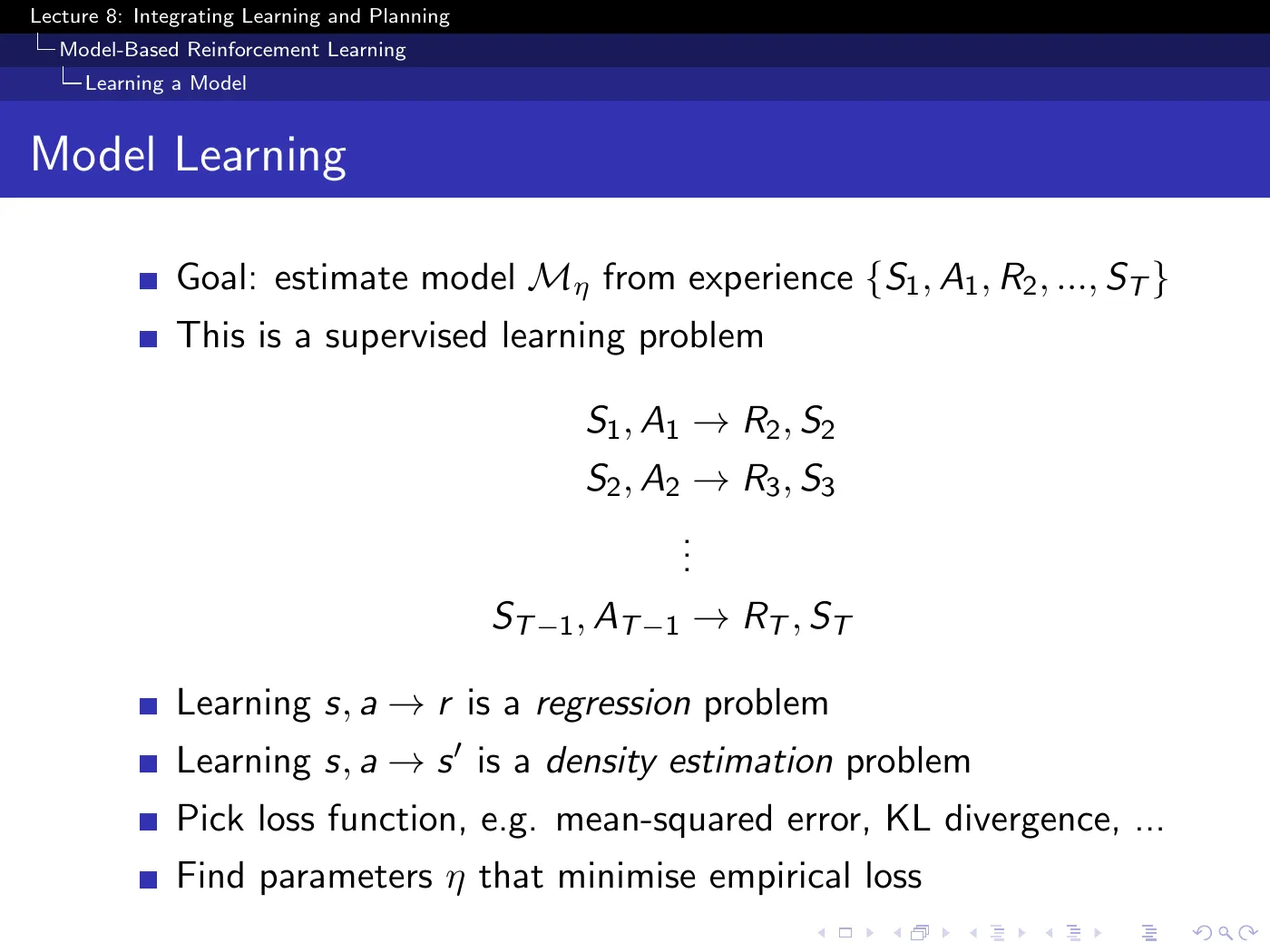
Lecture 8 Integrating Learning and Planning, slide 13

Model learning is supervised learning, and it splits into two problems of different type:

Target	Problem type	Typical loss
$s,a\to r$	regression	mean-squared error
$s,a\to s'$	density estimation	KL divergence

The structural problem that makes RL hard simply does not exist here

Every method in L4–L7 fought delayed, sparse credit: you act, and much later something good or bad happens, and you must work out what deserves the credit. That is what returns, bootstrapping, eligibility traces, and baselines were all for.
Model learning has none of it. You take one step and the environment immediately hands you the correct answer — this is the reward, this is the next state. There is a supervisor, the label arrives instantly, and there is no credit assignment problem at all.
That is the real content of "can efficiently learn model by supervised learning methods," and it is the strongest argument on p.11.

p.14–15 · Table Lookup Model ⏱ 27:33

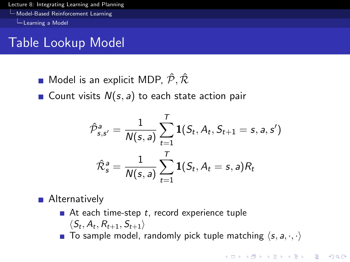
Lecture 8 Integrating Learning and Planning, slide 15

\hat{\mathcal{P}}^a_{s,s'}=\frac{1}{N(s,a)}\sum_{t=1}^{T}\mathbf{1}\{S_t=s,A_t=a,S_{t+1}=s'\}, \qquad \hat{\mathcal{R}}^a_s=\frac{1}{N(s,a)}\sum_{t=1}^{T}\mathbf{1}\{S_t=s,A_t=a\}R_{t+1}.

Ignore the indicator notation; it says count the transitions and average the rewards. This is the maximum-likelihood model.

The second bullet gives an equivalent non-parametric version: store every tuple $\langle S_t,A_t,R_{t+1},S_{t+1}\rangle$ and, to sample, draw uniformly from those matching $\langle s,a,\cdot,\cdot\rangle$ .

A replay buffer can act as a limited non-parametric model

The stored tuples have the same form as DQN's replay memory from L6. Replay samples transitions for learning updates; this table model samples conditioned on a particular state-action pair so that a simulated trajectory can continue.
The equivalence is exact only when matching samples exist. In continuous or rarely visited spaces, an ordinary replay buffer cannot answer an arbitrary $(s,a)$ query and therefore is not, by itself, a general simulator.

The two forms are parametric and non-parametric ends of the same spectrum. Under the slide's tabular expected one-step planning setup, either can support the same kind of backup. They are not information-identical: a tuple store retains empirical reward samples, whereas a count-and-mean model compresses them and can discard higher moments or transition–reward coupling. Everything else — linear, Gaussian, Gaussian process, deep network — sits between them and is primarily a supervised-learning choice.

3 · Planning by sampling

Robotics counterpart

Sampling-based MPC (MPPI, CEM, predictive sampling) plans the same way — sampled rollouts through a simulator from the current state — but aggregates rollout cost directly into an action choice instead of learning a value from the samples → MPC over a Learned Policy

p.16 · AB Example ⏱ 30:35

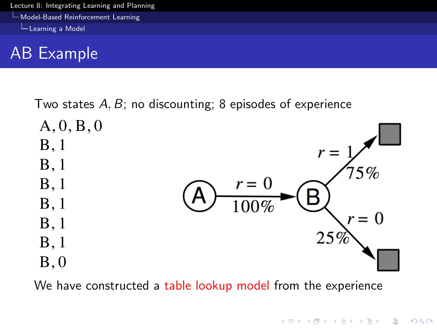
Lecture 8 Integrating Learning and Planning, slide 16

Counting gives $A\to B$ with $r=0$ at $100\%$ , and $B\to$ terminal with $r=1$ at $75\%$ and $r=0$ at $25\%$ . Nothing more than tallying.

This is the same eight episodes from L4 → Silver RL Lecture 4 — Question List, reused for a different purpose, and the reuse is the point.

p.17–19 · Sample-Based Planning ⏱ 32:52

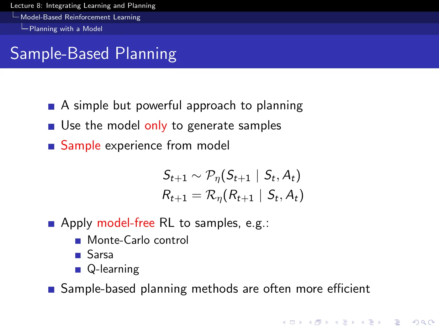
Lecture 8 Integrating Learning and Planning, slide 18

Use the model only to generate samples, then apply model-free RL to them. You are deliberately avoiding an explicit sum over all successor probabilities, not discarding the distribution itself.

That trade buys you the thing dynamic programming could never have: DP does a full-width backup over every possible successor, including ones with negligible probability. Sampling spends effort in proportion to what actually happens.

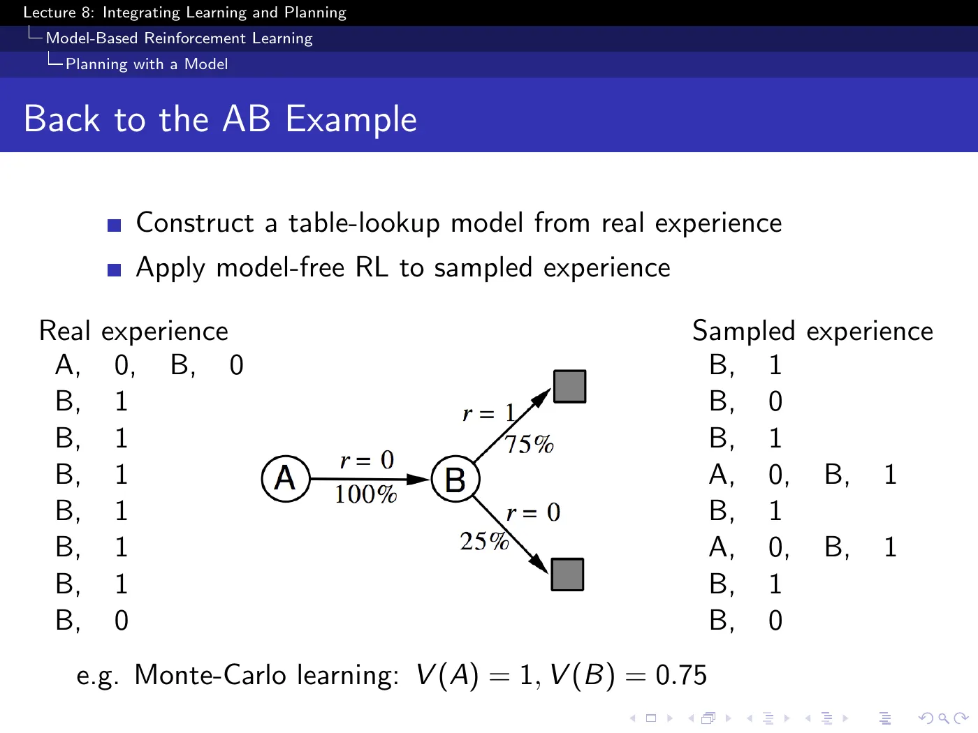
Lecture 8 Integrating Learning and Planning, slide 19

This is what TD learning was doing implicitly all along

In L4 the same eight episodes produced the canonical split: batch MC gives $V(A)=0$ , batch TD gives $V(A)=0.75$ → Silver RL Lecture 4 — Question List. MC fits the returns actually observed from $A$ — there was one, and it was $0$ . TD instead builds $\hat{\mathcal{P}},\hat{\mathcal{R}}$ and shares structure across states.
That $\hat{\mathcal{P}},\hat{\mathcal{R}}$ is precisely the table-lookup model on p.16. Batch TD(0) converges to the certainty-equivalence estimate — the value function that would be exactly right if the maximum-likelihood model were exactly right (Sutton & Barto 2e §6.3).
So model-based RL here is not a new answer. It is the same answer TD was already computing, arrived at explicitly instead of implicitly.

Then why did we ever need TD, if the model route reaches the same place?

Cost. Sutton & Barto put numbers on it: forming the maximum-likelihood model takes $O(n^2)$ memory in the number of states, and solving it conventionally takes $O(n^3)$ computation. The certainty-equivalence estimate is in a sense the optimal use of the data, and it is almost never feasible to compute directly.
TD approximates the same solution with $O(n)$ memory and repeated sweeps over the data. On large state spaces it may be the only feasible route to that solution.
Read the two lectures together and the relationship is clear: L4's TD is the cheap approximation, L8's model-based planning is the explicit computation, and which one you want depends entirely on the size of your problem.

The numbers on this slide are one small sample, not the answer

The slide reports $V(A)=1$ , $V(B)=0.75$ from the sampled episodes shown. $V(A)=1$ is sampling noise — the two sampled $A$ -episodes happened to end in $r=1$ .
The model's actual implied value is $V(A)=0+V(B)=0.75$ . Sample more and you converge there. Do not memorize $V(A)=1$ .

4 · When the model is wrong

p.20 · Planning with an Inaccurate Model ⏱ 44:20

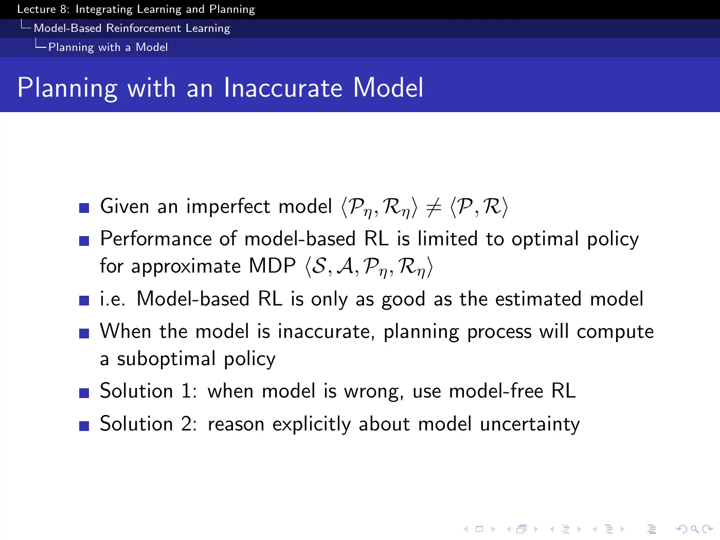
Lecture 8 Integrating Learning and Planning, slide 20

The bound is exact and worth stating in one line: your performance ceiling is the optimal policy of the MDP you believe in, not of the one you are in. Perfect planning on a wrong model yields the right answer to the wrong question.

This should not be alarming on its own. Every method in this course is approximate somewhere; model-based RL has simply relocated the approximation from the value function to the dynamics. Sometimes that is a better place for it.

The two remedies are both worth remembering, because they organize the rest of the lecture and the next one:

When the model is wrong, fall back on model-free RL — which is Dyna, in section 5.
Reason explicitly about model uncertainty — the Bayesian route, deferred here and adjacent to L9.

Model uncertainty is an exploration tool, not just a caveat

A model tells you what you know. That means it also tells you what you do not know — and you can deliberately act to visit states whose dynamics you understand badly.
That is a fundamentally different exploration mechanism from $\epsilon$ -greedy, which perturbs randomly with no notion of what would be informative. It is one of the genuine advantages of being model-based, and the lecture flags it without developing it.

5 · Dyna

p.22–25 · Real and Simulated Experience ⏱ 48:07

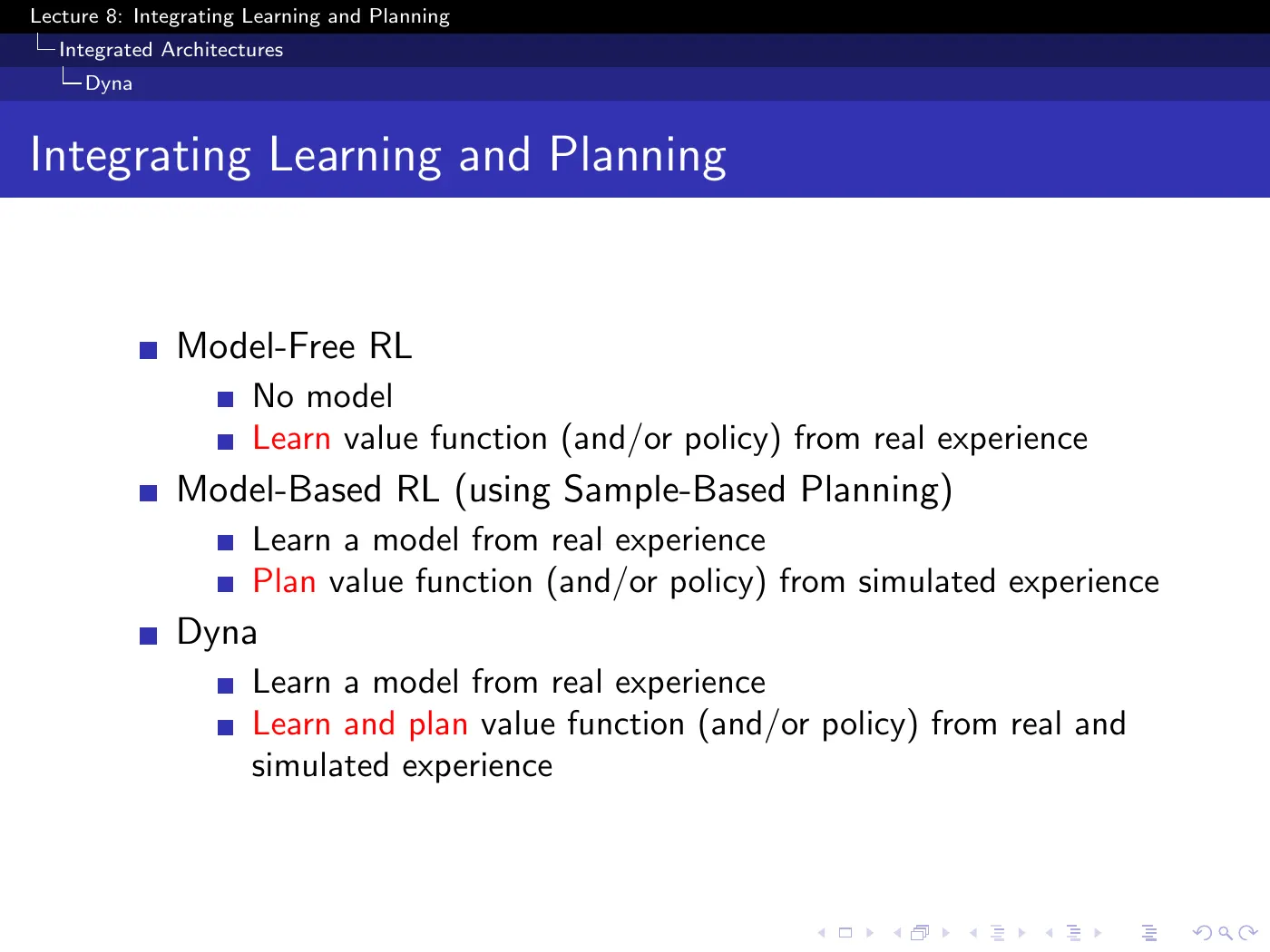
Lecture 8 Integrating Learning and Planning, slide 25

Two sources of experience, and Dyna's answer to which to use is simply: both. Real experience is scarce and trustworthy; simulated experience is abundant and only as good as the model. There is no reason to discard either.

Can the direct-RL arc ever make things worse?

Yes. Real transitions are trustworthy samples but still noisy, and direct updates can interfere with a value function improved by deep search. Conversely, simulated updates can dominate with model bias. Dyna specifies that both sources are used, not an optimal weighting between them. Dyna-2 (p.52) keeps long- and short-term estimates separate, but the lecture does not prove that this separation can never hurt.

p.26–27 · Dyna Architecture and Dyna-Q ⏱ 53:28

Lecture 8 Integrating Learning and Planning, slide 26

Lecture 8 Integrating Learning and Planning, slide 27

Steps (d) and (f) are the same update

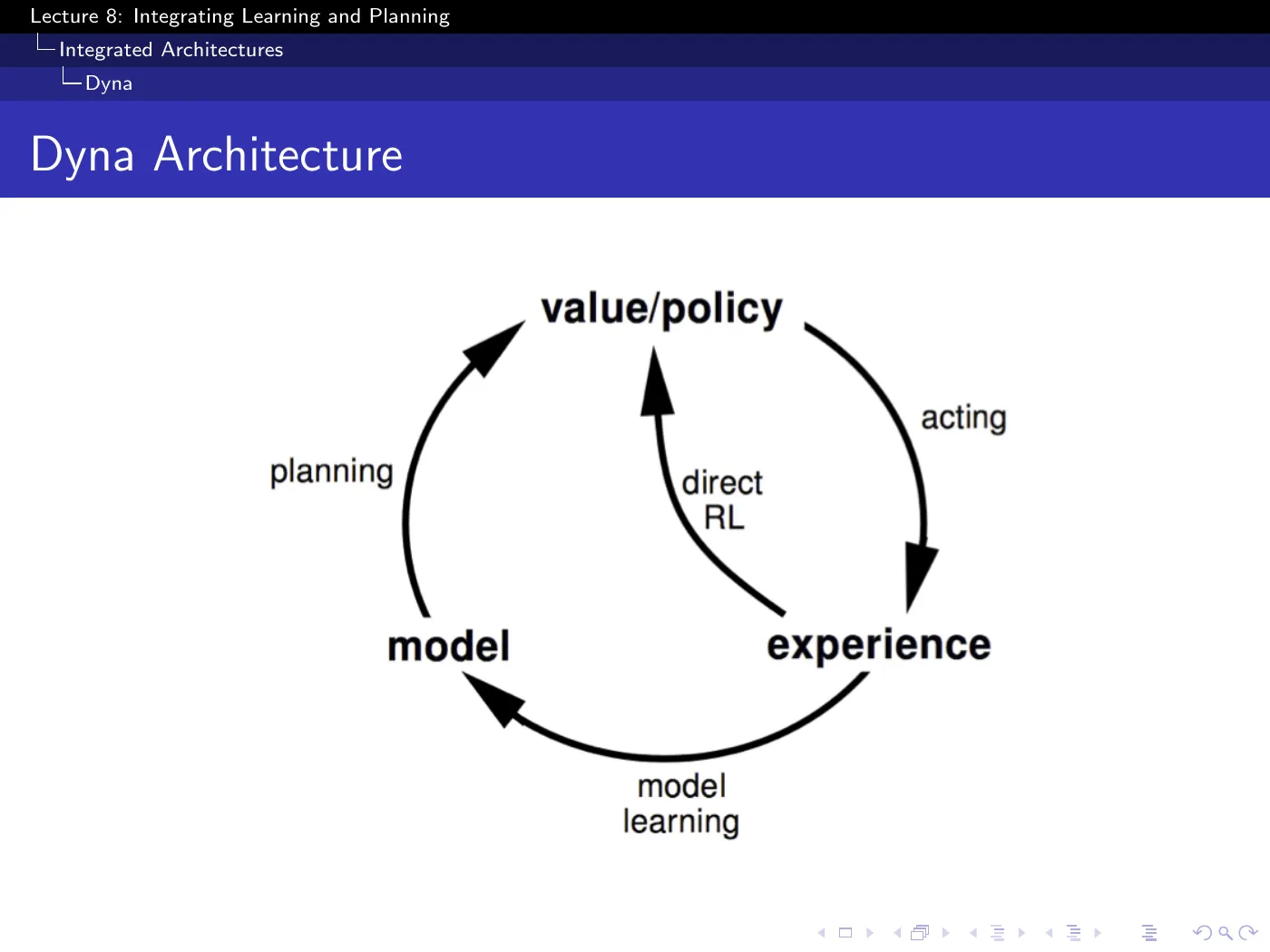
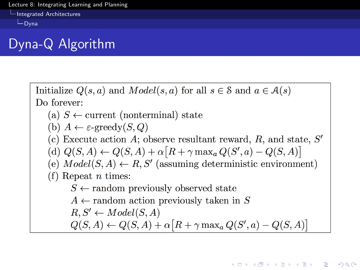
Look at the pseudocode: step (d) is a Q-learning update on a real transition, and the update inside the step (f) loop is a Q-learning update on an imagined one. Character for character, the same equation.
Dyna is Q-learning plus a model and a loop that feeds the model's output back into the same learner. The architecture can be paired with other update rules, but policy and off-policy assumptions must still match; replacing Q-learning with Sarsa or actor-critic is not automatically consequence-free.

Step (f) is the thinking loop, and $n$ is how much thinking you do per real step. Note the parenthetical on step (e): the model update shown assumes a deterministic environment, since it simply overwrites $Model(S,A)\leftarrow R,S'$ rather than accumulating counts.

The acting rate and the thinking rate are independent budgets. You act as often as the world requires and think as much as the time between actions allows — planning as an anytime procedure.

p.28 · Dyna-Q on a Simple Maze ⏱ 56:35

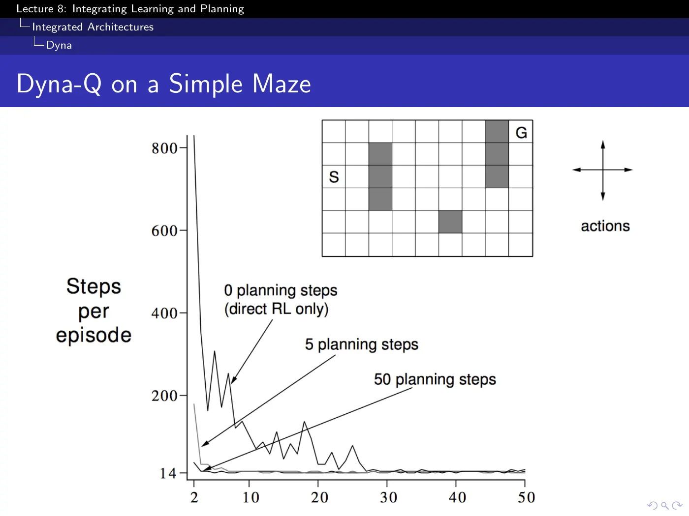
Lecture 8 Integrating Learning and Planning, slide 28

Y-axis is steps per episode, so lower is better, and $14$ is optimal. With $n=0$ (pure model-free) it takes roughly 30 episodes; with $n=5$ it is nearly converged within a couple.

The mechanism behind that gap is not on the slide. A single stumbling first episode already reveals many one-step transitions. Replaying them from the model lets value information propagate backwards through the maze without physically re-walking it. Model-free learning must actually traverse each transition, repeatedly, to back the values up the same distance.

On this maze, Dyna gains nothing within the first episode

There is no reward until the goal is reached, so before the first success there is simply no information to propagate and nothing for planning to do.
With an earlier penalty, one bad transition can be replayed many times and its value propagated through other already observed predecessor transitions. A tabular Dyna model does not invent unobserved nearby transitions from one sample; that extra generalization would require a function approximator or structured model.

p.29–30 · Dyna-Q with an Inaccurate Model ⏱ 1:01:08

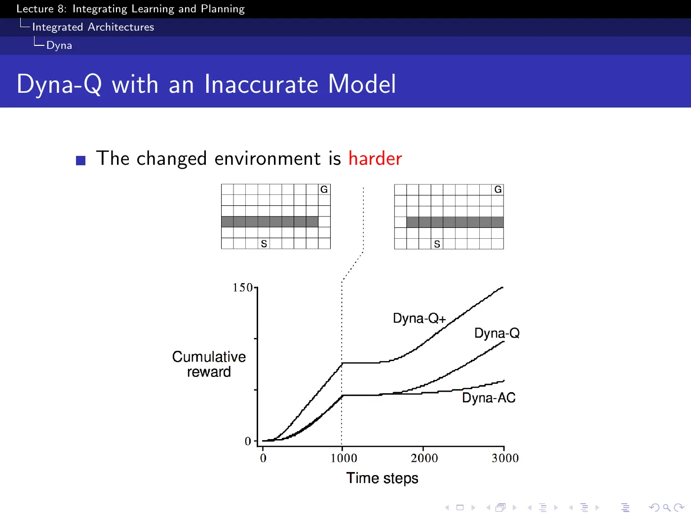
Lecture 8 Integrating Learning and Planning, slide 29

The environment changes mid-run: the gap in the barrier moves. What follows is the concrete failure mode of p.20.

The flatline is the lesson

After the change the curve goes flat. The agent is not merely uninformed — it is actively planning against a stale model that insists the old route works, and spending its whole thinking budget rehearsing a path that no longer exists.
A wrong model can give a confident, well-optimized answer to a world that no longer exists. A tabular model-free agent avoids this particular planning failure, although stale values, function approximation, and insufficient exploration can still make model-free learning slow or wrong in their own ways.

Dyna-Q+ recovers faster because it adds an exploration bonus to state-action pairs not tried recently, which pushes the agent to re-check actions whose consequences may have changed.

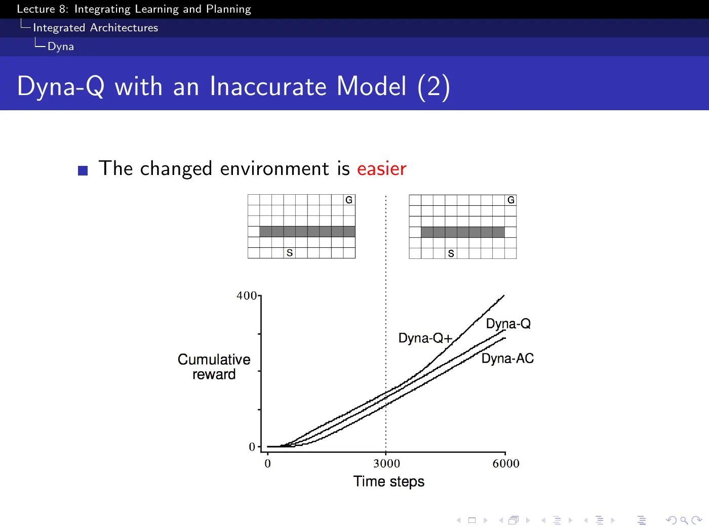
Lecture 8 Integrating Learning and Planning, slide 30

The "easier" case is the harder one — and the asymmetry is the interesting part

Here a shortcut opens rather than a route closing. Plain Dyna-Q may never find it, and the reason is precise: its current path still works. Nothing goes wrong, no error signal appears, and there is no pressure to look. It keeps collecting a decent score forever while a better option sits unexamined.
Only the exploration bonus finds it. Blocked paths announce themselves; missed opportunities do not.

6 · Forward search

p.32–34 · Forward Search and Simulation-Based Search ⏱ 1:04:57

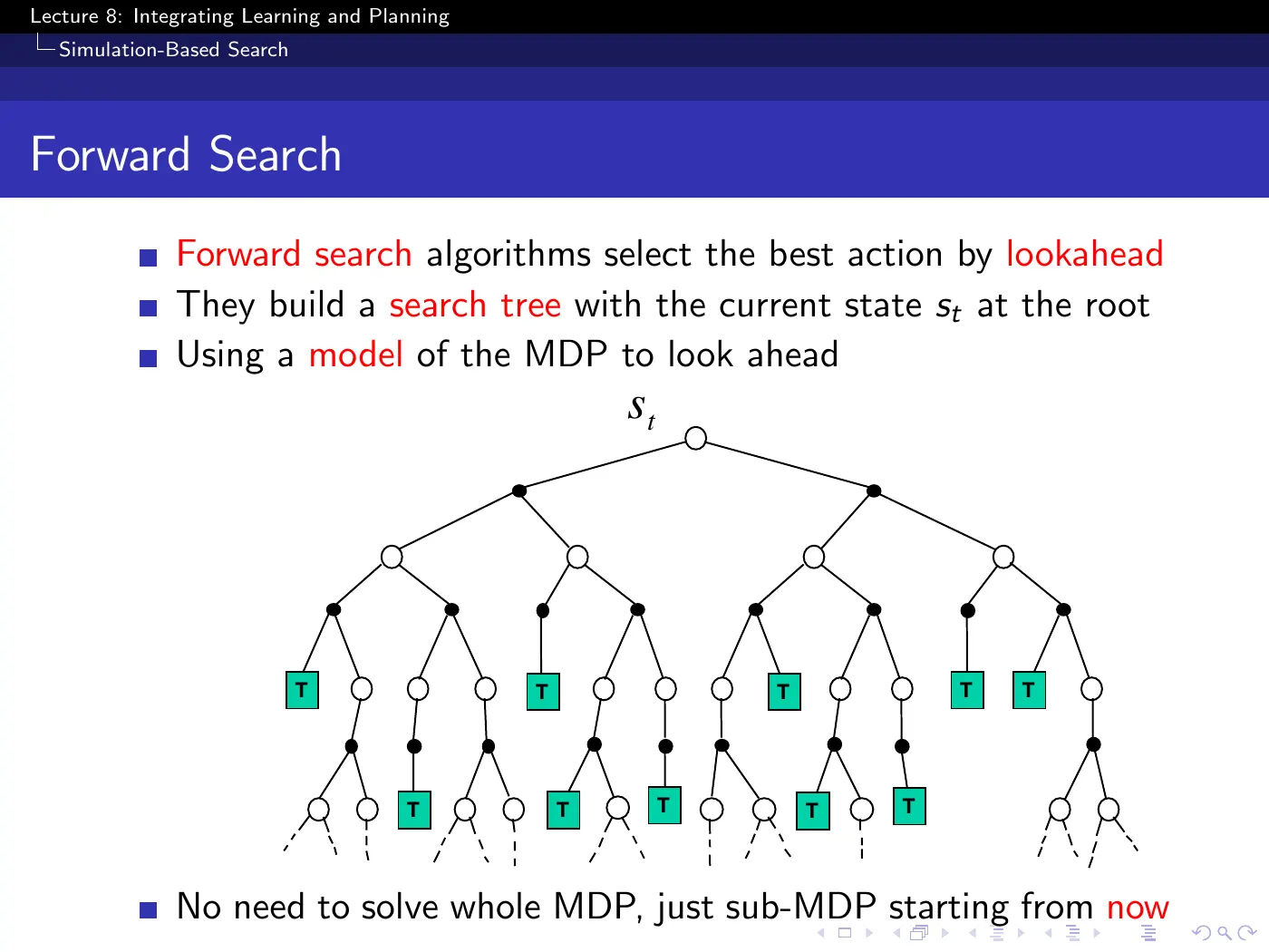
Lecture 8 Integrating Learning and Planning, slide 32

Dyna sampled transitions from anywhere in the state space. Forward search makes the opposite bet: one state matters far more than the others, and it is the one you are standing in.

Solve the sub-MDP from now, not the MDP

You do not need the optimal policy for states you will not reach for a year, or may never reach. You need the right action here. Rooting a search tree at $s_t$ and looking forward turns a possibly intractable problem into a small one, and the reduction can be dramatic.
This is the sharpest structural idea in the lecture, and it is what separates planning from solving.

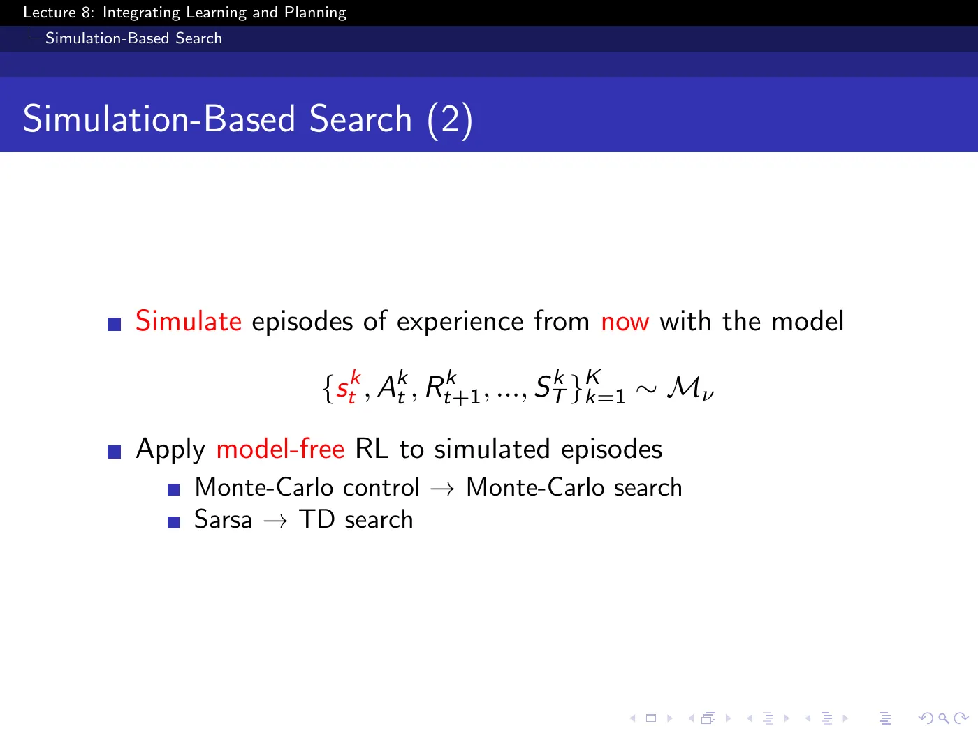
Lecture 8 Integrating Learning and Planning, slide 34

\{s^k_t,A^k_t,R^k_{t+1},\dots,S^k_T\}_{k=1}^{K}\sim\mathcal{M}_\nu

Simulation-based search is the intersection of the two ideas: forward search for where to look, sampling for how to look there. Then apply model-free RL to what comes back — Monte-Carlo control gives Monte-Carlo search, Sarsa gives TD search.

Note the second win from sampling. It focuses effort twice over: on actions you would plausibly choose, and on outcomes the environment would plausibly produce.

p.35 · Simple Monte-Carlo Search ⏱ 1:11:05

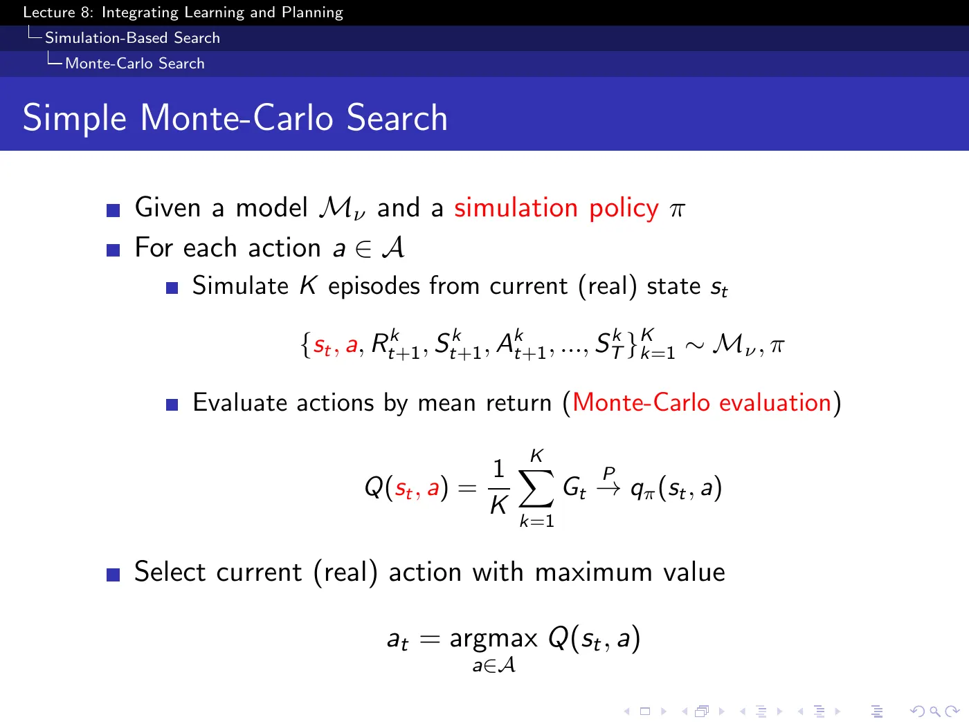
Lecture 8 Integrating Learning and Planning, slide 35

The stripped-down version: for each action available at the root, run $K$ simulations under a fixed simulation policy $\pi$ , average the returns, pick the best. With independent rollouts from the stated model and finite expected returns, the law of large numbers makes each average converge to that model's $q_\pi(s_t,a)$ .

Two limitations, both fixed on the next slide: the simulation policy never improves, and only the root actions get evaluated. Everything the simulations pass through on the way is thrown away.

7 · Monte-Carlo tree search

p.36–37 · MCTS Evaluation and Simulation ⏱ 1:14:08

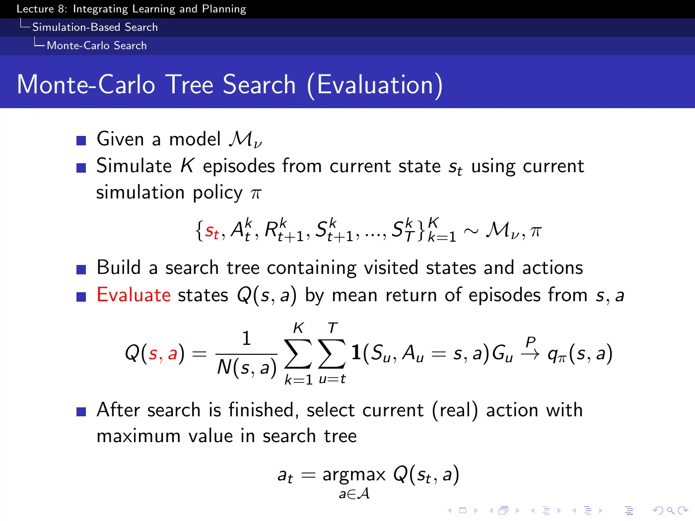
Lecture 8 Integrating Learning and Planning, slide 36

Q(s,a)=\frac{1}{N(s,a)}\sum_{k=1}^{K}\sum_{u=t}^{T}\mathbf{1}(S_u,A_u=s,a)\,G_u\;\xrightarrow{P}\;q_\pi(s,a)

The change from p.35 is that every visited state-action pair gets a value, not just the root ones. The simulations were passing through all that structure anyway; MCTS keeps it.

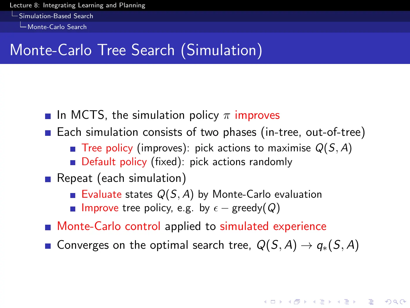
Lecture 8 Integrating Learning and Planning, slide 37

MCTS is L5's Monte-Carlo control, pointed at imagined experience

Evaluate by Monte-Carlo, improve by $\epsilon$ -greedy, repeat. That is GLIE Monte-Carlo control from L5, run on simulated episodes rooted at the current state.
The slide's convergence claim $Q\to q_*$ reuses the same logic: returns evaluate visited actions, while persistent exploration and increasingly greedy selection improve the tree policy. The conditions still matter — a finite search problem, enough visits to relevant actions, and returns sampled from the stated model. Finite-budget MCTS is an approximation, not an exact planner.

The two-phase split follows directly from that framing. Inside the tree you have $Q$ values, so you can act greedily — the tree policy, which improves. Outside the tree you have nothing, so you fall back on a fixed default policy, typically uniform random. The tree boundary is simply the frontier of what you have learned.

The rollouts use a crude policy. Doesn't that bias everything above them?

At finite search budgets, yes. As simulations accumulate and the tree expands, more of the return is generated by the improving tree policy and less by the fixed default policy. Under the lecture's finite-tree and persistent-exploration assumptions, that influence vanishes asymptotically; it is not a free guarantee for arbitrary continuous or indefinitely deep problems.
In practice the choice of rollout policy matters a great deal for how fast this happens — but even uniform random rollouts work strikingly well. Random is less dumb than it sounds when you are averaging over enough of it.

p.38–41 · Go ⏱ 1:18:39

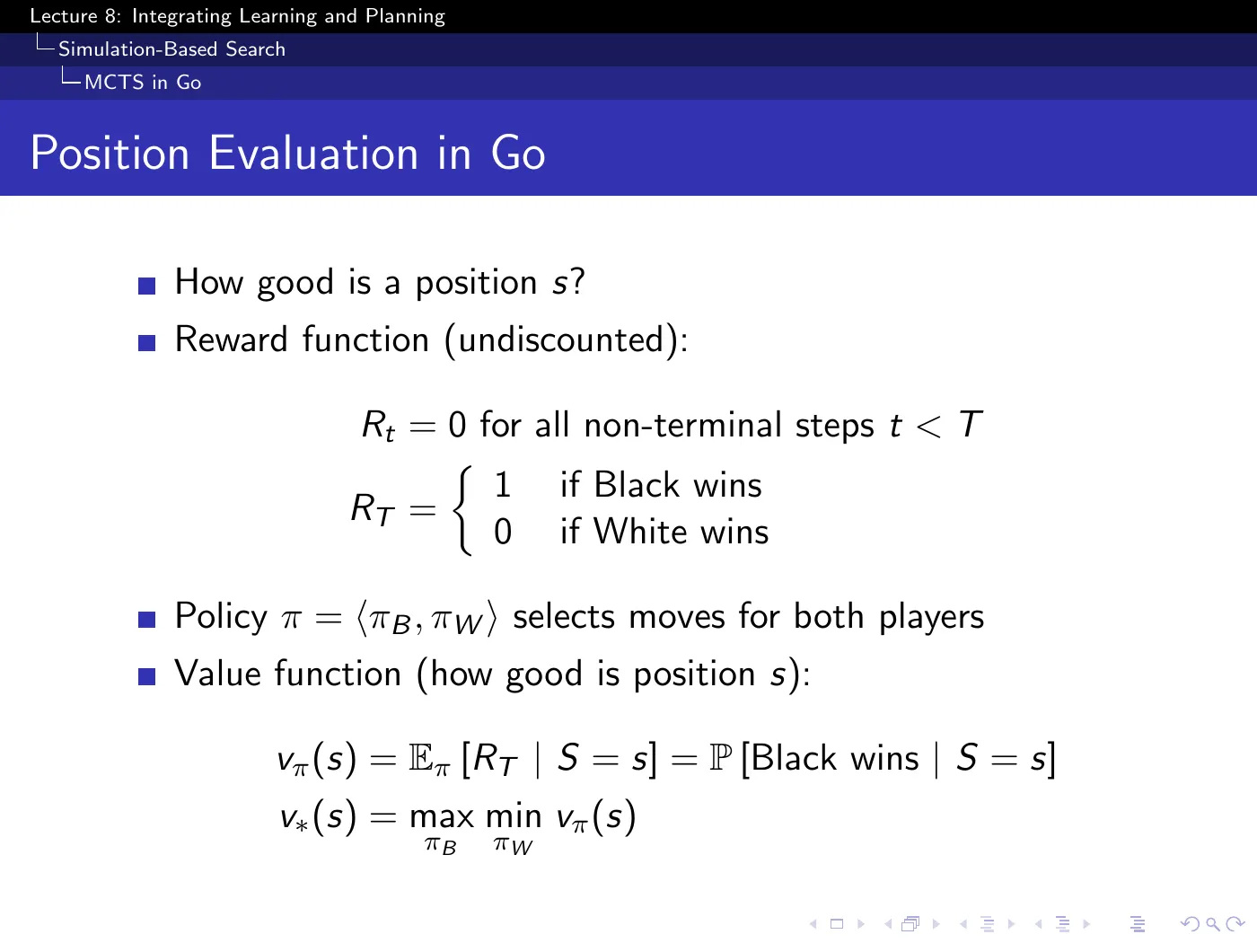
Lecture 8 Integrating Learning and Planning, slide 40

v_\pi(s)=\mathbb{E}_\pi[R_T\mid S=s]=\mathbb{P}[\text{Black wins}\mid S=s], \qquad v_*(s)=\max_{\pi_B}\min_{\pi_W}v_\pi(s)

With reward $0$ throughout and $1/0$ at the end, the value function is literally a win probability. That is worth pausing on — the expectation of a $0/1$ indicator is a probability, so "how good is this position" and "how likely am I to win" become the same number rather than merely analogous.

The optimal value is a $\max\min$ because there are two players. That is the one place the RL formalism needs a twist for games, and it is deferred to L10.

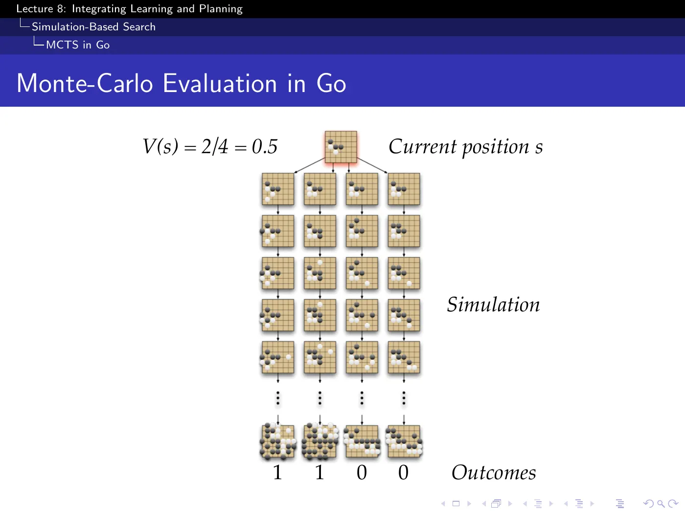
Lecture 8 Integrating Learning and Planning, slide 41

Two wins out of four rollouts gives $V(s)=0.5$ . Crude beyond belief — and hard to beat.

Why a naive rollout beats a sophisticated value function

Silver's remark, which is on no slide: careful function approximation struggles to outperform this, because a learned $\hat v$ must be right about the entire state space, while a rollout estimate probes this position, now, dynamically.
Search buys you specialization. You spend your whole compute budget on the one state that matters instead of amortizing it over states you will never see.

p.42–46 · MCTS Walkthrough ⏱ 1:23:11

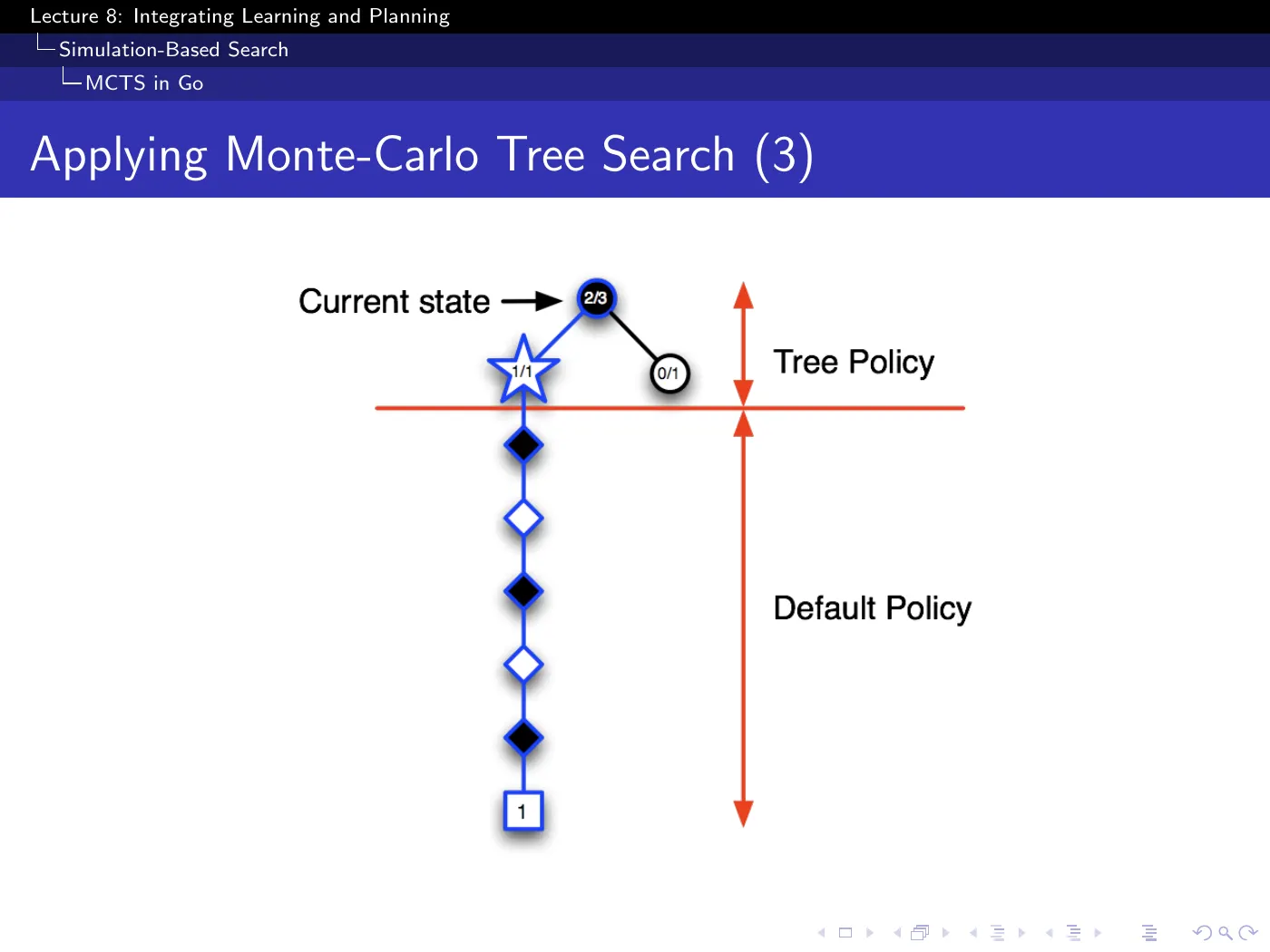
Lecture 8 Integrating Learning and Planning, slide 44

Reading the notation: star = a state being added to the tree for the first time, diamond = passed through during an out-of-tree rollout and not stored, square = terminal, with $1$ meaning Black won. Each simulation's result is backed up along the whole path, so counts at the root accumulate as $1/1$ , $1/2$ , $2/3$ , $2/4$ …

The behavior to notice across the five slides is that the tree grows asymmetrically. Promising lines get developed deeply; unpromising ones are left as stubs. This is best-first search, and each simulation restarts at the root and re-chooses, so earlier commitments are continuously revisited.

The exploration caveat is the same as everywhere else in this course: you must keep sampling the apparently-bad branches a little, or you will never discover that one of them was misjudged.

p.47–48 · Advantages, and Go Strength ⏱ 1:27:43

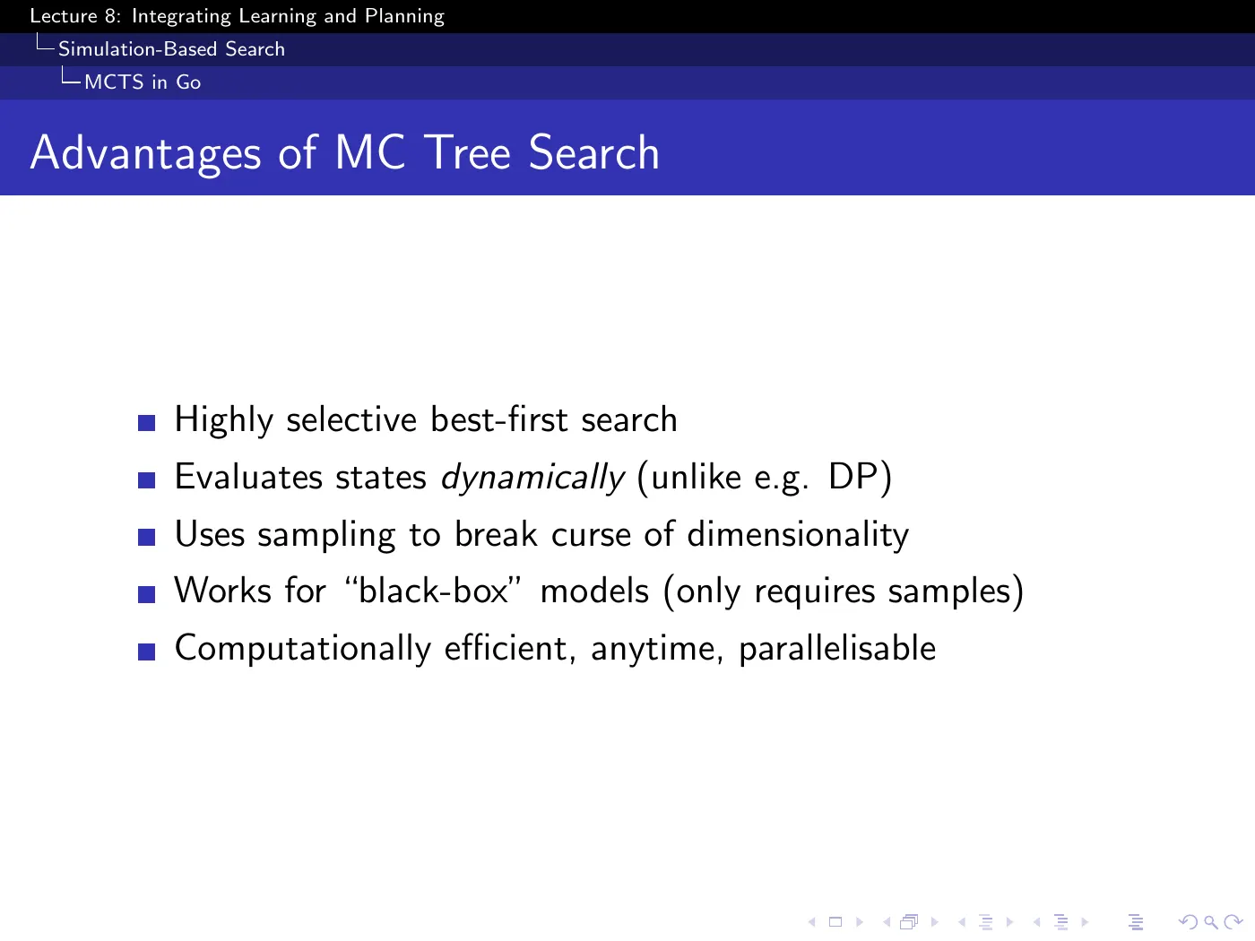
Lecture 8 Integrating Learning and Planning, slide 47

The bullet worth extracting: works for black-box models. MCTS never asks for $\mathcal{P}^a_{ss'}$ — it only needs something that, given a state and action, produces a next state. A simulator, a game engine, a physics package, or a learned network all qualify equally. That is a much weaker requirement than dynamic programming's, and it is why the method transferred so readily across domains.

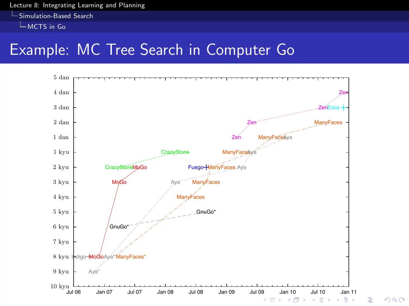
Lecture 8 Integrating Learning and Planning, slide 48

Read this axis carefully — it runs in two directions

The y-axis is the Go ranking system: kyu ranks count down as you improve (9 kyu → 1 kyu), then dan ranks count up (1 dan → 9 dan). So the whole plot is "better as you go up" only because the kyu labels are printed in descending order.
Calibration: one rank difference means that if the stronger player gave the weaker one a free move, they would be evenly matched.

The step change around 2006–2007 is MoGo and CrazyStone arriving — the first Monte-Carlo search programs — after which every program on the chart is a Monte-Carlo program. Classical brute-force search had simply stalled in Go.

8 · TD search and Dyna-2

p.49–51 · TD Search ⏱ 1:31:32

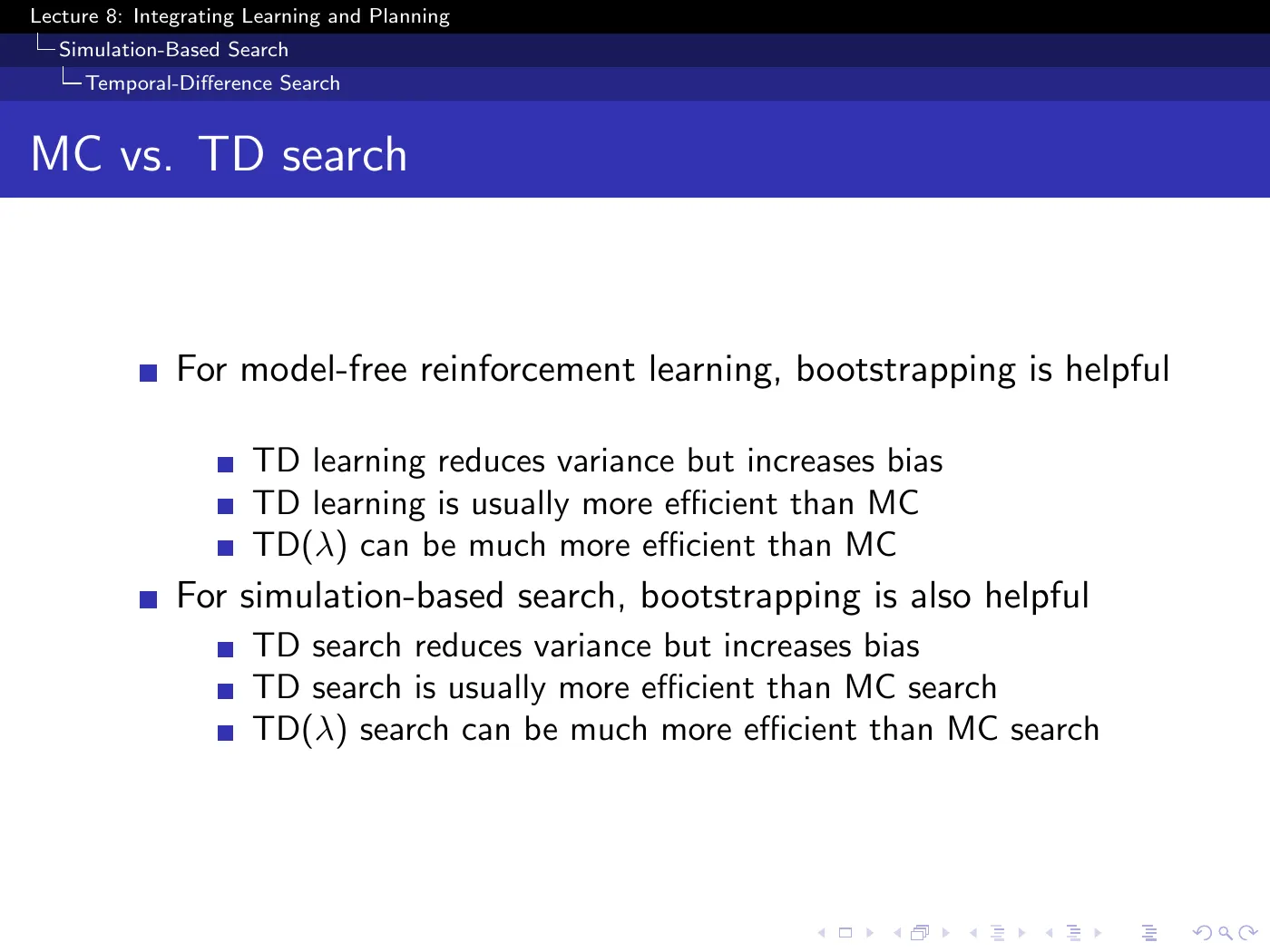
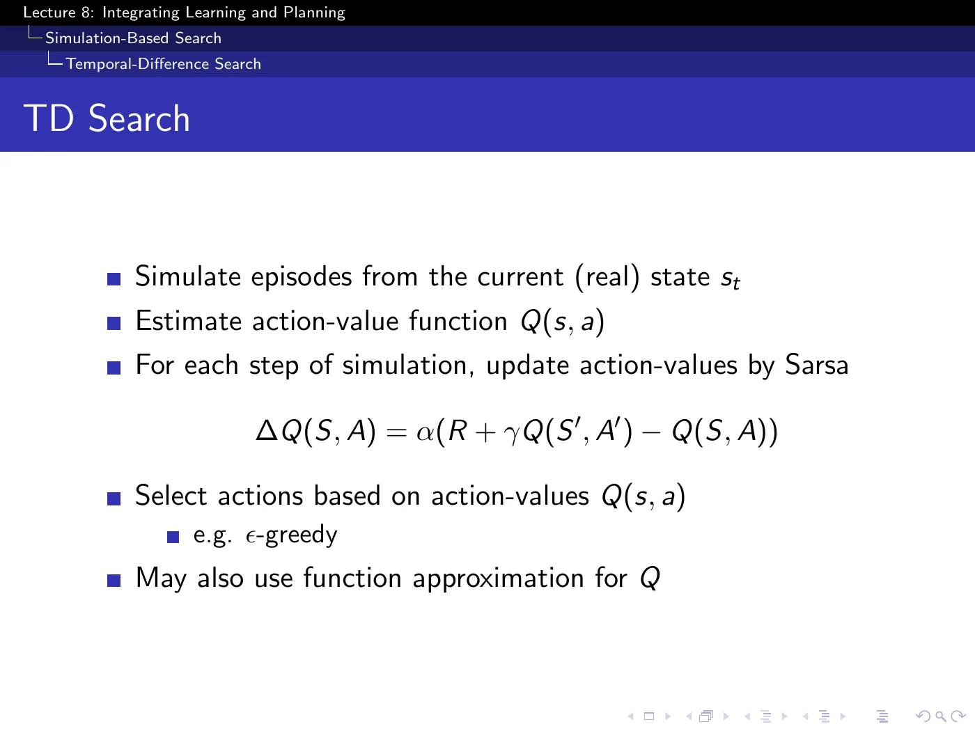
Lecture 8 Integrating Learning and Planning, slide 50

Q(S,A)\leftarrow Q(S,A)+\alpha\big(R+\gamma Q(S',A')-Q(S,A)\big)

The substitution is mechanical: MCTS applies Monte-Carlo control to the sub-MDP from now; TD search applies Sarsa to it. Everything else stays.

The justification is transplanted wholesale from L4–L6 — bootstrapping reduces variance at the cost of bias, is usually more efficient, and TD( $\lambda$ ) can be much better than either extreme. p.50 simply asserts that what was true for learning is also true for search.

Lecture 8 Integrating Learning and Planning, slide 51

When TD search beats MC search — the condition is not on any slide

Bootstrapping pays off when the same state can be reached by many different paths, i.e. when your search space is a graph rather than a strict tree.
If you already learned something about a state by arriving through one line of play, bootstrapping lets you reuse it the moment you arrive by another. In a strict tree every node is reached exactly one way and there is nothing to share, so the advantage disappears.
That is the structural test for whether to reach for TD search, and Go — where transpositions abound — is exactly the favorable case.

The last bullet is also easy to miss: nothing forces you to store $Q$ in a tree. Search values can live in a function approximator, which is what you need when the state space is too large for a table even locally.

p.52–53 · Dyna-2 ⏱ 1:35:21

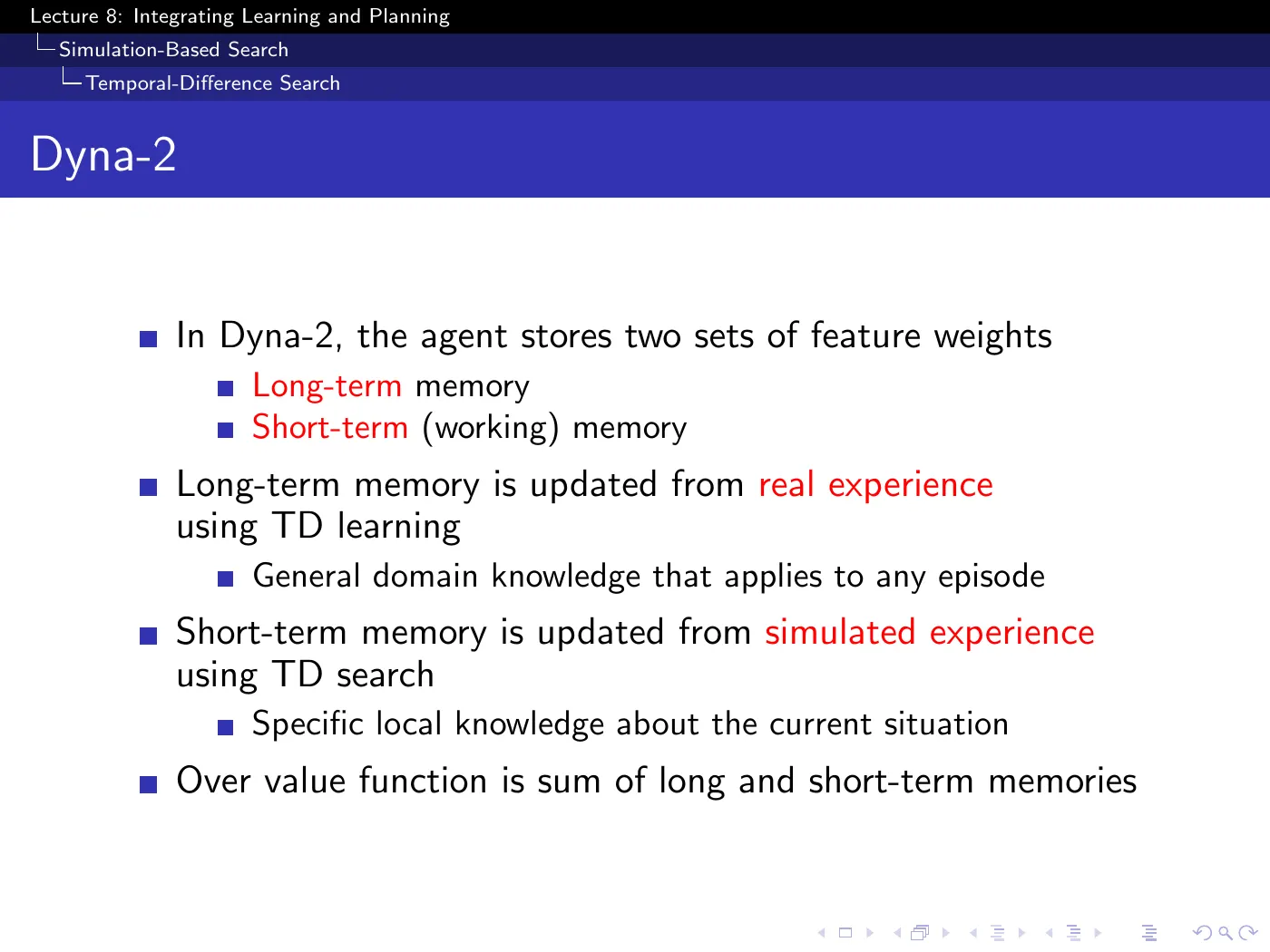
Lecture 8 Integrating Learning and Planning, slide 52

Two sets of weights, updated from the two sources of experience, and summed:

Memory	Updated from	Holds
Long-term	real experience, via TD learning	general knowledge that applies in any episode
Short-term (working)	simulated experience, via TD search	specific knowledge about the situation you are in now

The search tree is the short-term memory

Dyna-2 is Dyna's "use both sources" idea applied to forward search, with one addition that matters: the two estimates are kept separate rather than being written into the same table.
Separation prevents situation-specific search updates from directly overwriting the long-term parameters. It does not by itself prove that their sum is always better; it gives the architecture a clean way to retain reusable knowledge while rebuilding local search information for the current situation.

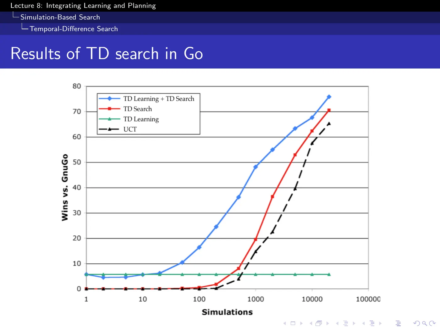
Lecture 8 Integrating Learning and Planning, slide 53

Four lines, and the comparison is unusually clean because the update rule, the representation of $Q$ , and the features are held identical across three of them. Only what experience they run on differs.

TD Learning (flat, ~5%) — learns the whole Go state space offline. It is flat because it does not use simulations at all, so more thinking time buys it nothing. This is the cost of trying to be right everywhere.
TD Search — the same updates applied to simulated experience rooted at the current position. It overtakes UCT and climbs steeply. Specialization wins.
UCT (dashed) — Monte-Carlo tree search, the benchmark.
Dyna-2 (highest) — both memories combined.

The most informative part of the plot is the left edge

At one simulation — before any thinking has happened — Dyna-2 already sits at the TD Learning baseline while TD Search and UCT start at zero. General knowledge pays off before you have thought at all, and search then builds on top of it rather than starting from nothing.
That is the whole argument for combining the two, made visible: not that either is better, but that they contribute at different points on the time axis.

Study checklist

Close the note and answer these in your own words. Reopen only the section linked after the question.

What new object is learned in L8, and what new budget does it create? → 1 · Why bother learning a model
Why are simulated transitions abundant but not independent new evidence? → The one idea
Distinguish learning $\mathcal P$ , learning $\mathcal R$ , and learning a value function. → 2 · What a model is, and how to learn one
What does sample-based planning avoid computing explicitly? → 3 · Planning by sampling
Under what assumptions does batch TD match the certainty-equivalence estimate in the AB example? → p.17–19 · Sample-Based Planning ⏱ 32:52
What two errors can compound in model-based RL? → 4 · When the model is wrong
In Dyna-Q, what is identical between the real and simulated updates, and what differs? → p.26–27 · Dyna Architecture and Dyna-Q ⏱ 53:28
Why is an opened shortcut harder to discover than a newly blocked route? → p.29–30 · Dyna-Q with an Inaccurate Model ⏱ 1:01:08
How do forward search and sampling reduce planning cost in different ways? → 6 · Forward search
What assumptions sit behind the slide's MCTS convergence claim? → 7 · Monte-Carlo tree search
When can TD search reuse more information than MC search? → p.49–51 · TD Search ⏱ 1:31:32
What do Dyna-2's long- and short-term memories each retain? → p.52–53 · Dyna-2 ⏱ 1:35:21

Gaps to close on your own

Unusually for this course, no slide in this deck is skipped — the lecture covers all 54 pages. The gaps are things named and deferred rather than pages passed over.

Bayesian model-based RL. Promised in the lecture as bonus slides ("we won't get to today"), and they are not in this deck at all — there is no Bayesian material anywhere in the 54 pages. This is the principled version of remedy 2 on p.20: keep a posterior over models rather than a maximum-likelihood point estimate, and act to reduce your uncertainty. It connects directly to L9.
UCT — defined in L10, not here. It appears as a line label on p.53 and as the standard MCTS benchmark, with the tree policy left as "smarter strategies using Bandits". L9 does not supply it either — that lecture develops UCB1 for bandits only. L10 p.37 finally states it: UCT is MCTS in which every node of the tree is treated as its own bandit problem, with UCB1 selecting among children, and self-play UCT converges on the minimax values for perfect-information zero-sum two-player games. That is the missing explanation for the asymmetric, best-first growth described above. For the regret analysis go to Kocsis & Szepesvári (2006).
Function approximation inside search. Stated explicitly: nothing forces search values into a tree or table, and a function approximator can help a great deal. Deferred for time, with a Civilization example mentioned but not shown.
Dyna-2 details. The architecture is described and the result shown, but the actual update rules and how the two memories are combined are not given.
Learning the state space. Assumed known throughout. Silver concedes the raw inputs may be useless for predicting dynamics and that learning your own representation is typically a good idea — which is what modern model-based deep RL is largely about.
How to weight real against simulated experience. Dyna says "use both" and the lecture concedes that combining them badly can hurt, and that combining them well requires estimating how reliable each source is. No method for doing that is given here; Dyna-2's separate memories are the closest the lecture comes.

Language notes

Phrasings worth stealing for your own technical writing and talks:

Expression	Use
the agent's model of the world	naming an internal representation without overclaiming
break open the trajectory	use intermediate structure rather than one end-of-run number
breaks the curse of dimensionality	a method that avoids exponential blow-up by sampling
only as good as the model we've learned	stating a performance ceiling in one clause
an anytime procedure	usable whenever interrupted, better if given longer
a reasonable proxy	a stand-in that is wrong but useful
asymptotically any bias we introduce gets removed	conceding an approximation while bounding its cost
isn't as dumb as you might think	defending a naive baseline that empirically works
these things happen at their natural rates	two coupled processes with independent clocks
we've given something up, but it gains us something	framing a deliberate trade-off