Lecture 4 · Model-Free Prediction

Slides: David Silver - RL Course (UCL 2015) · Previous: Lecture 3 · Planning by Dynamic Programming · Next: Lecture 5 · Model-Free Control
Companion: Silver RL Lecture 4 — Question List (your own stuck points, in Korean) · Model-Free Prediction · Forward and Backward Views of TD Lambda

Read this instead of watching. Each slide is embedded below with only what the slide itself does not say — the reasoning, the caveats, and the questions worth being able to answer.

The one idea

L3 solved a known MDP with dynamic programming. L4 takes the model away and keeps the goal: given a policy, how good is each state?

Everything in the lecture is one question asked at different depths:

How far into the real trajectory do you look before you substitute your own guess for the rest?

Look ahead	Target	Method
all the way to termination	$G_t$	Monte-Carlo
one step	$R_{t+1}+\gamma V(S_{t+1})$	TD(0)
$n$ steps	$G_t^{(n)}$	$n$ -step TD
a geometric blend of every $n$	$G_t^\lambda$	TD( $\lambda$ )

Every algorithm in the rest of the course has one shape

The incremental-mean rewrite on p.10 is not a computational convenience — it is the template:

\text{new estimate} \leftarrow \text{old estimate} + \alpha\big(\underbrace{\text{target}}_{\text{what happened}}-\underbrace{\text{old estimate}}_{\text{what you predicted}}\big)

MC puts $G_t$ in the target slot, TD(0) puts $R_{t+1}+\gamma V(S_{t+1})$ , TD( $\lambda$ ) puts $G_t^\lambda$ . L5 puts $Q$ -targets there, L6 multiplies by a gradient, L7 by a score function. Learn to read the target slot and the whole course becomes one algorithm.

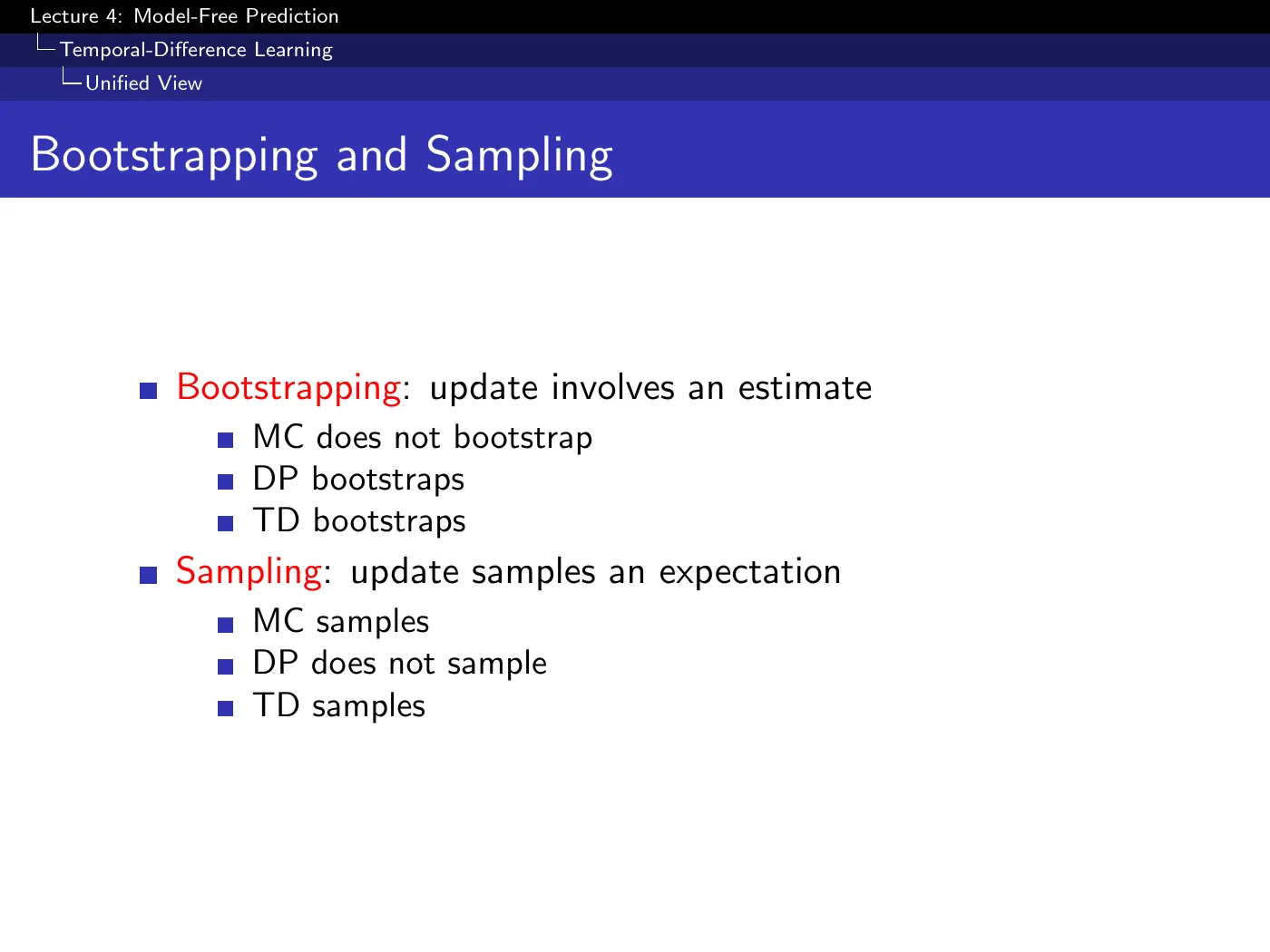
Two independent axes, four algorithms

p.29 splits the design space along two questions that have nothing to do with each other:

Do you bootstrap? (does the target contain your own estimate) — MC no, TD yes, DP yes.
Do you sample? (or expand the full expectation) — MC yes, TD yes, DP no.

	full-width	sample
no bootstrap	exhaustive tree search	Monte-Carlo
bootstrap	dynamic programming	TD

DP and MC are not opposites; they differ on both axes. TD is the corner that takes one property from each, which is why it is the most practical and the least well-behaved.

1 · Monte-Carlo policy evaluation
2 · Incremental updates
3 · Temporal-difference learning
4 · Bias and variance
5 · What they converge to
6 · The unified view
7 · n-step returns
8 · TD-lambda, forward view
9 · TD-lambda, backward view
Study checklist
Gaps to close on your own
Language notes

1 · Monte-Carlo policy evaluation

p.3–5 · Model-Free Prediction ⏱ 2:15

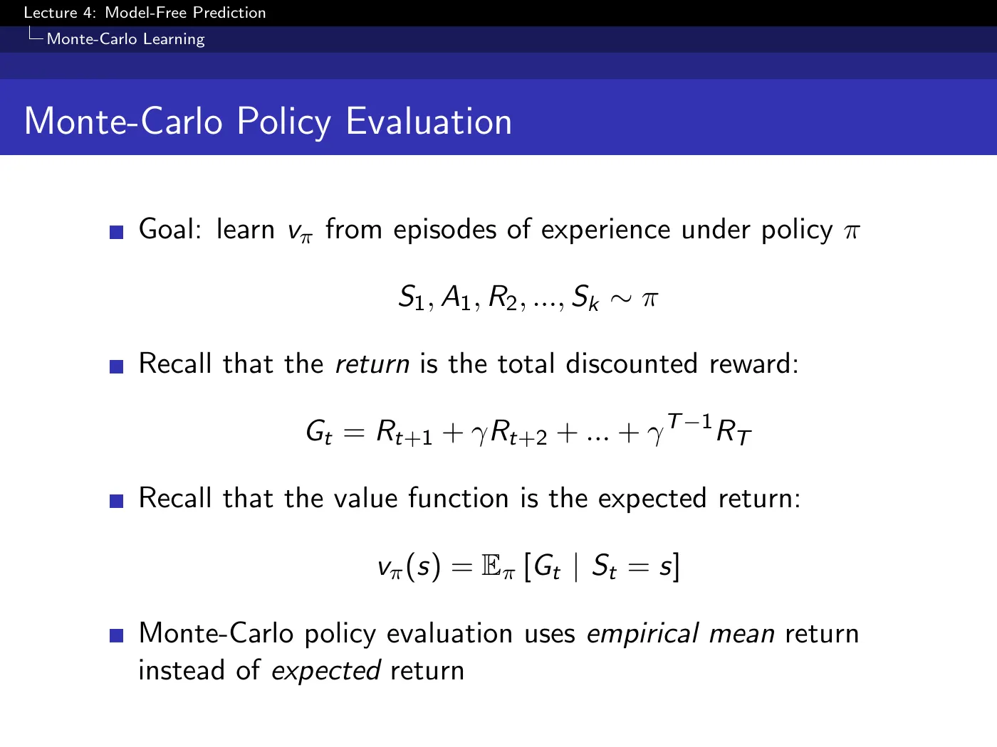
Lecture 4 Model-Free Prediction, slide 5

The assumption being dropped is stated on p.3 and is worth feeling the weight of: nobody hands you $\mathcal{P}$ and $\mathcal{R}$ . For any interesting system — a factory, a helicopter, a game whose opponent you did not write — writing down the transition dynamics is not merely tedious, it is unavailable.

The structure of the response mirrors L3 exactly. L3 split into evaluate a policy then use that to find the best policy. L4 does the first half without a model; L5 does the second.

v_\pi(s)=\mathbb{E}_\pi[G_t\mid S_t=s]\;\longrightarrow\;\text{empirical mean of observed }G_t

That substitution — expectation → empirical mean — is the entire Monte-Carlo idea. Everything else on the next few slides is bookkeeping about how to collect the samples.

p.6–7 · First-Visit and Every-Visit MC ⏱ 9:01

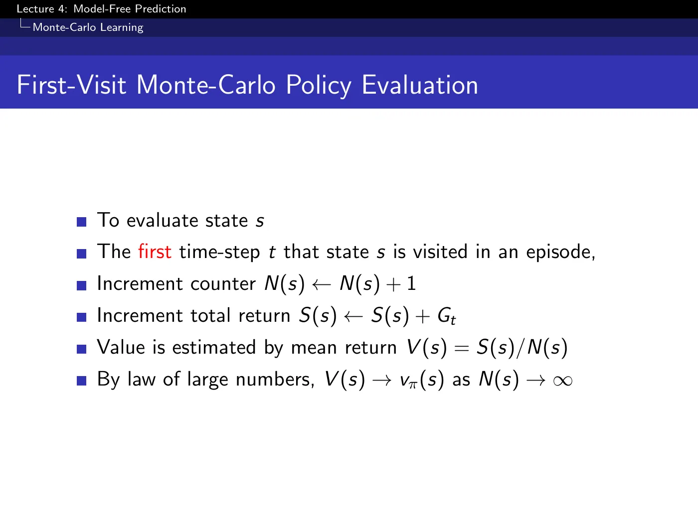
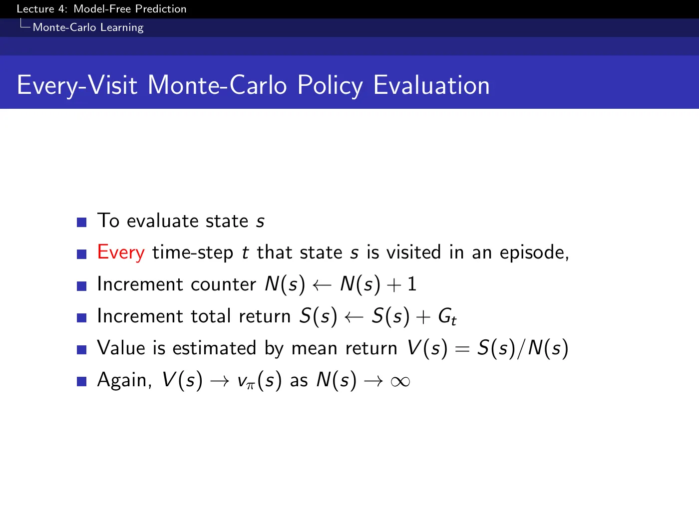
Lecture 4 Model-Free Prediction, slide 6

Lecture 4 Model-Free Prediction, slide 7

The two differ only in what happens when a trajectory revisits a state: count it once, or count every visit with its own (different) return.

$N(s)$ and $S(s)$ persist across episodes. The slide's increment notation invites reading them as per-episode counters; they are not. You are accumulating a mean over the whole run.

Both are consistent by the law of large numbers, and the lecture declines to declare a winner — the choice reappears in L4's own backward view as accumulating versus replacing traces, and the evidence favors each in different domains.

Why sampling breaks the curse of dimensionality

The convergence rate follows from the central limit theorem: the error variance shrinks like $1/N(s)$ — where $N(s)$ is the number of visits to that state, not the number of states in the MDP.
So the cost of estimating one state's value is completely independent of how large the state space is. DP had to sweep every state on every iteration; MC only pays for the states it actually visits, in proportion to how often the policy visits them.
That is the structural reason model-free methods scale where dynamic programming cannot, and it is stated in the lecture but on no slide.

p.8–9 · Blackjack ⏱ 16:37

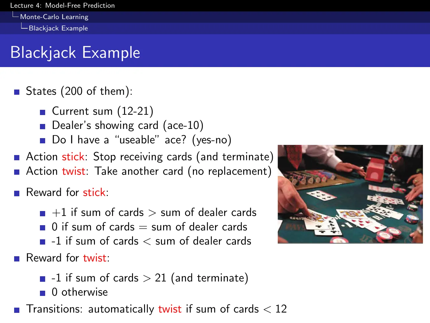
Lecture 4 Model-Free Prediction, slide 8

200 states from three variables: current sum (12–21), dealer's showing card (ace–10), usable ace (yes/no). Sums below 12 are excluded because there is no decision to make — you always twist, so the MDP auto-twists and those states are not part of the problem.

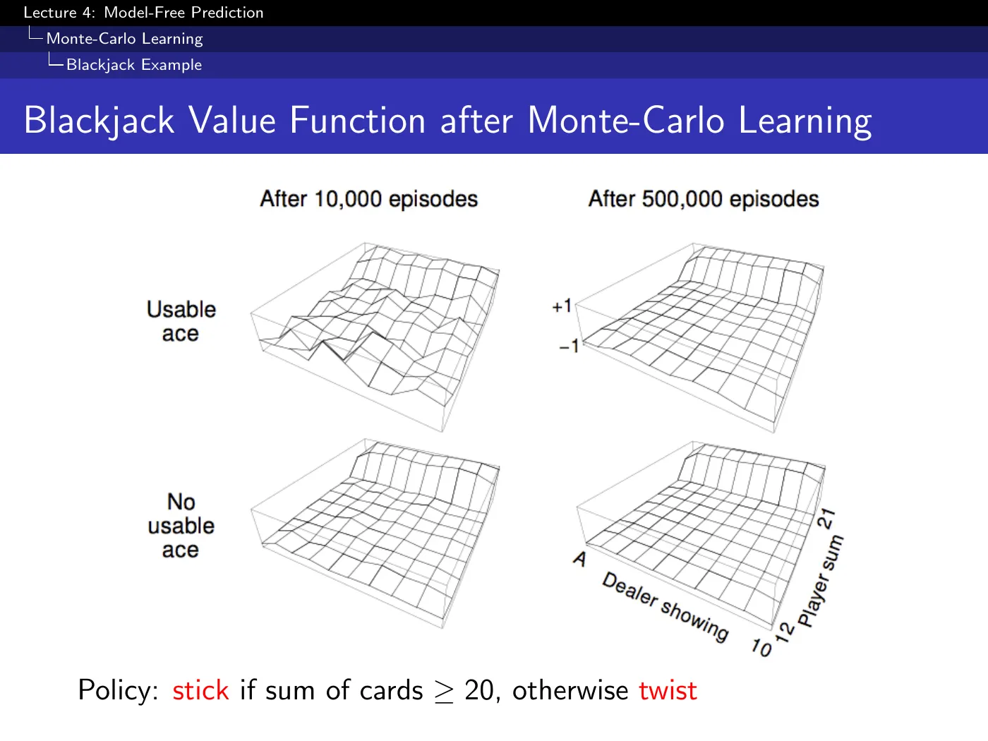
Lecture 4 Model-Free Prediction, slide 9

The two panels differ in noise for a reason worth generalizing

After 10,000 episodes the no usable ace surface is already smooth while the usable ace surface is visibly noisy, and it takes around 500,000 episodes to settle. Nothing is wrong with the algorithm — usable-ace states are simply rarer, so 10,000 hands do not deliver enough visits to each.
The lesson generalizes past blackjack: your sample complexity is set by visitation frequency per state, not by episode count. A rare-but-important region of the state space will stay wrong long after the common regions look converged.

The shape itself is worth reading: the value drops sharply below a sum of 20 because the policy is deliberately naive (stick only on 20–21, otherwise twist), so it keeps twisting into a bust.

And the point of the whole example: nobody told the agent the deck composition, the dealer's strategy, or any transition probability. The value function depends on all of them and was recovered anyway, from sampled play alone.

2 · Incremental updates

p.10–11 · Incremental Mean and Incremental MC ⏱ 26:29

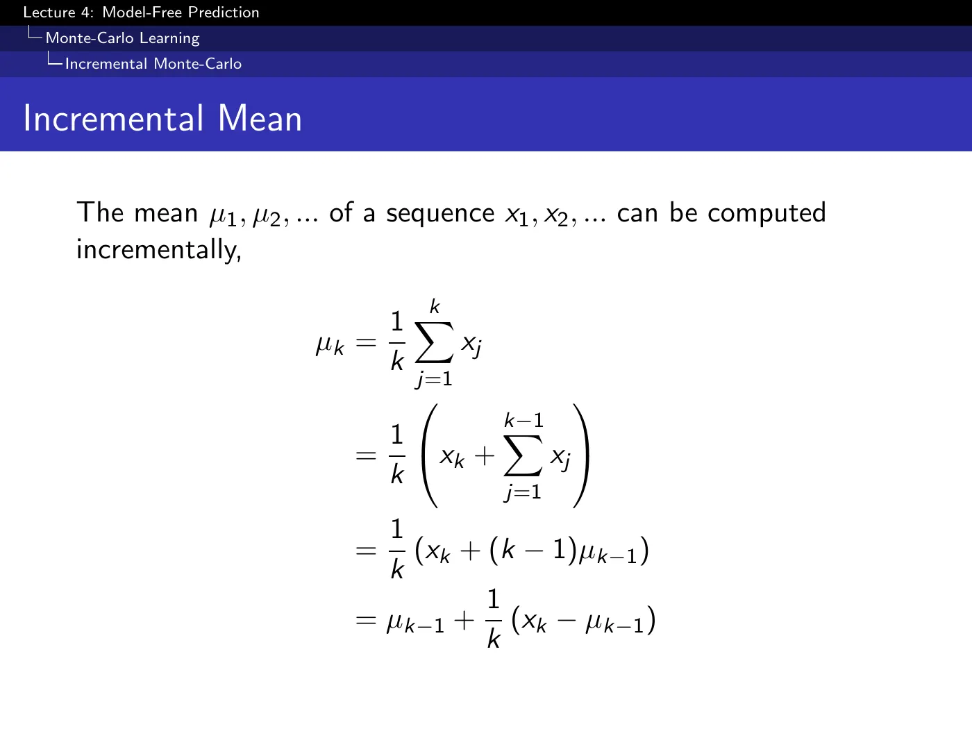
Lecture 4 Model-Free Prediction, slide 10

\mu_k=\mu_{k-1}+\frac{1}{k}\big(x_k-\mu_{k-1}\big)

Algebraically trivial and structurally the most important line in the lecture — it is the template quoted at the top of this note. Read the three parts as prediction, error, correction.

Lecture 4 Model-Free Prediction, slide 11

V(S_t)\leftarrow V(S_t)+\frac{1}{N(S_t)}\big(G_t-V(S_t)\big) \qquad\text{or}\qquad V(S_t)\leftarrow V(S_t)+\alpha\big(G_t-V(S_t)\big)

Constant

\alpha

is not an approximation of

1/N

— it is a different estimator, and you will almost always want it

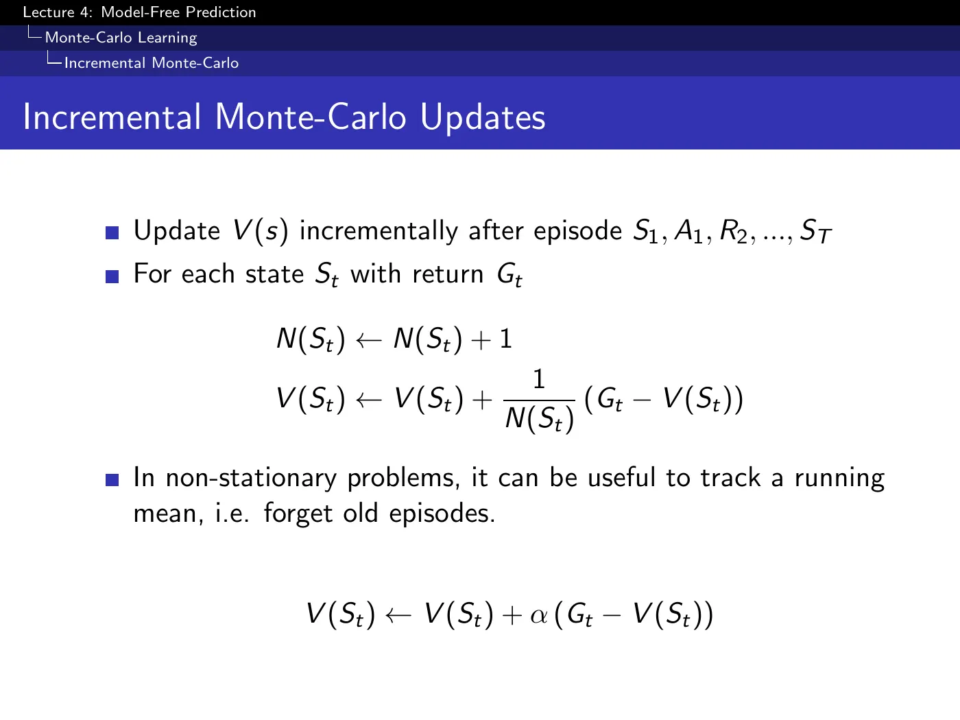
With $1/N$ you compute the true running mean of everything ever seen. With constant $\alpha$ you compute an exponentially weighted moving average that forgets the past at a fixed rate.
The slide's justification is "non-stationary problems". The lecture supplies the reason that actually matters: in control you are always non-stationary. From L5 onward the policy keeps improving, so returns collected early came from a worse policy and are actively misleading. Averaging them in with full weight is not conservatism, it is baggage.
This is the same $1/N$ -versus- $\alpha$ distinction that decides whether initialization matters at all → Lecture 5 · Model-Free Control.

"Incremental" here still means per episode. You must reach the end of the episode to know $G_t$ before you can update anything. Removing that constraint is the next section.

3 · Temporal-difference learning

p.12–13 · TD(0) ⏱ 34:07

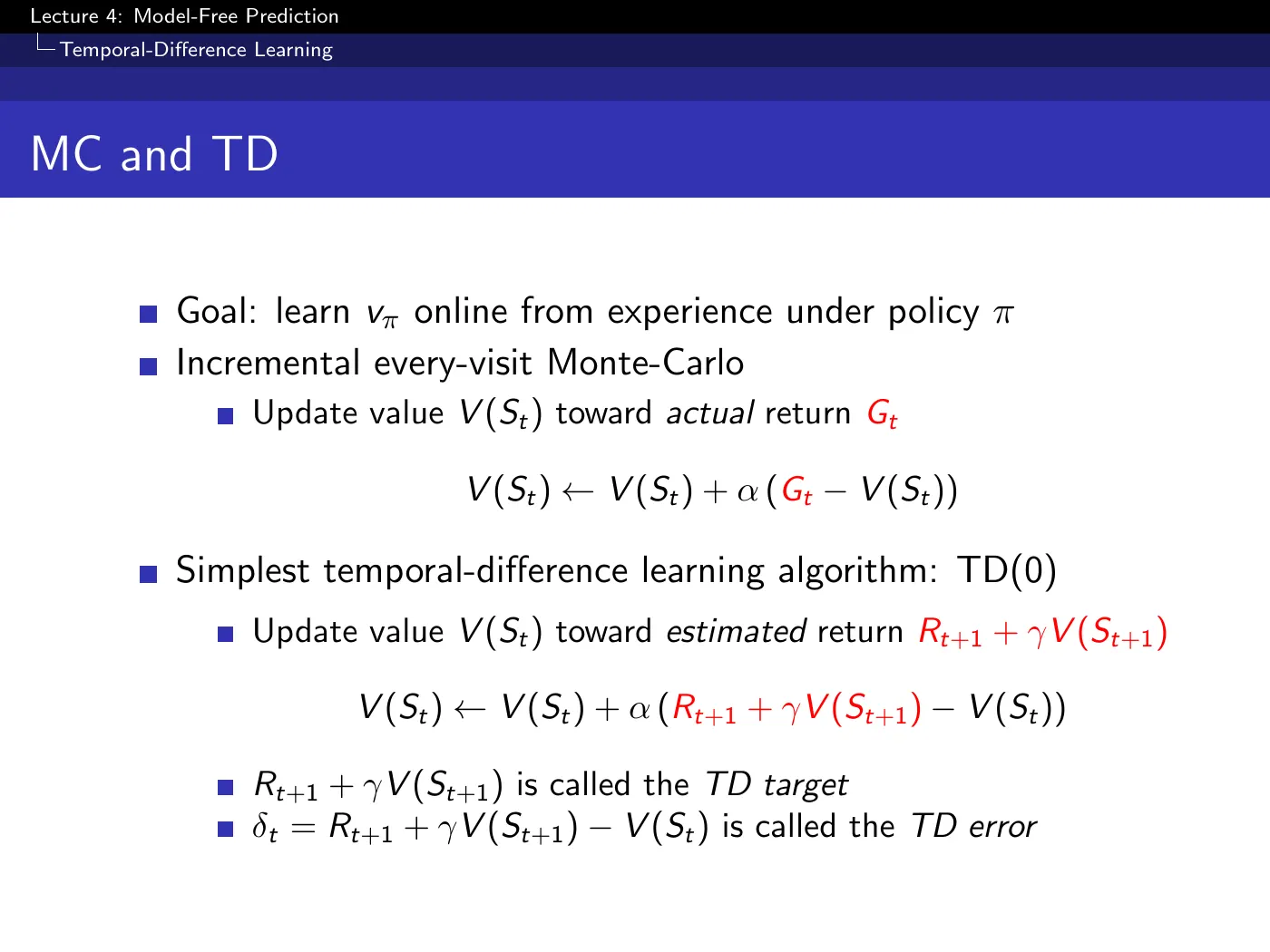
Lecture 4 Model-Free Prediction, slide 13

V(S_t)\leftarrow V(S_t)+\alpha\big(\underbrace{R_{t+1}+\gamma V(S_{t+1})}_{\text{TD target}}-V(S_t)\big), \qquad \delta_t=R_{t+1}+\gamma V(S_{t+1})-V(S_t)

One substitution in the target slot: the real return becomes one real step plus your own estimate of the rest. Bootstrapping — "update a guess towards a guess."

The near-crash, which is the best argument for bootstrapping in the course

You are driving. A car hurtles toward you, you are certain you are about to crash — and at the last second it swerves and nothing happens.
Monte-Carlo learns nothing from this. No crash occurred, so the return contains no penalty, and the state where you were about to die gets no negative signal.
TD learns immediately. Your estimate went from "fine" to "about to die" in one step, which is a large TD error, and it updates the earlier state right then: that situation was worse than I thought — I should have slowed down.
You do not have to die to learn that you nearly died. Bootstrapping lets a change in prediction be a learning signal in its own right, rather than requiring an outcome.

p.14–15 · Driving Home ⏱ 39:27

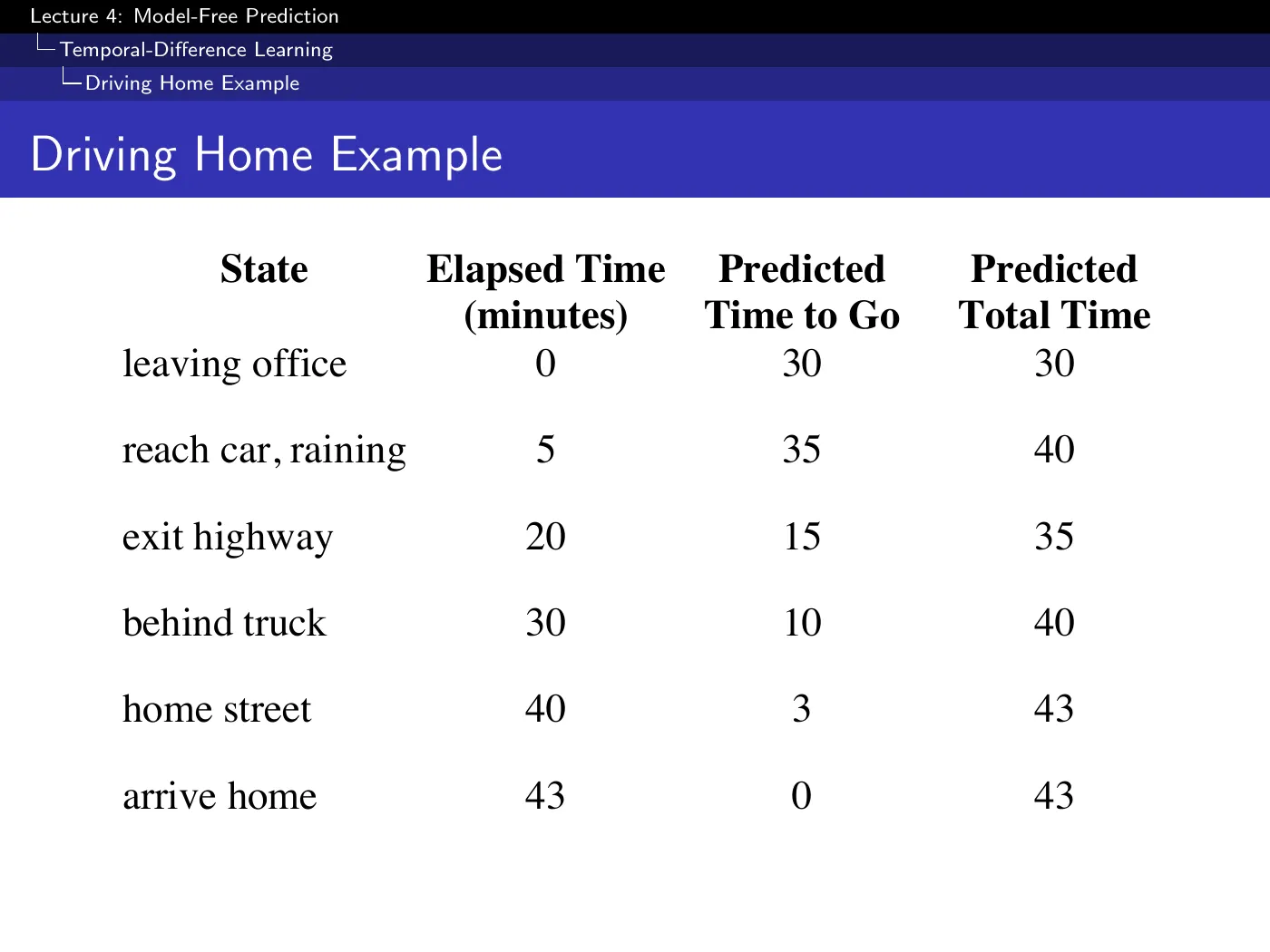
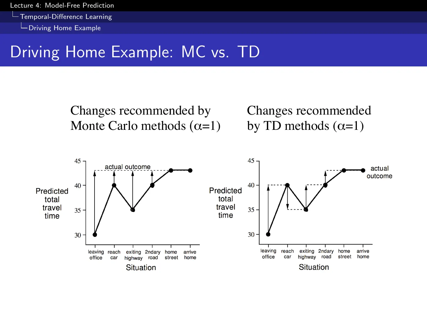
Lecture 4 Model-Free Prediction, slide 14

Lecture 4 Model-Free Prediction, slide 15

Read the arrows, because the two panels are the whole distinction:

MC (left): every point's arrow points at the same place — the final 43 minutes — and none of them can be drawn until the drive is over.
TD (right): each point's arrow points at the next prediction, and each can be drawn the moment the next estimate exists.

"It started raining" is information about the total journey time that arrives at minute 5. MC discards it until minute 43; TD uses it at minute 5.

What the reward function is in this example

There are no actions here — this is a Markov reward process, not an MDP. That is not a simplification of convenience: any MDP with a fixed policy flattens into an MRP, and prediction is exactly the problem of evaluating that MRP.
The reward is elapsed time (negate it, and "get to work fast" becomes maximizing reward with $-1$ per step). Actions only start mattering in L5, when you begin choosing them.

4 · Bias and variance

p.16–18 · MC versus TD ⏱ 44:45

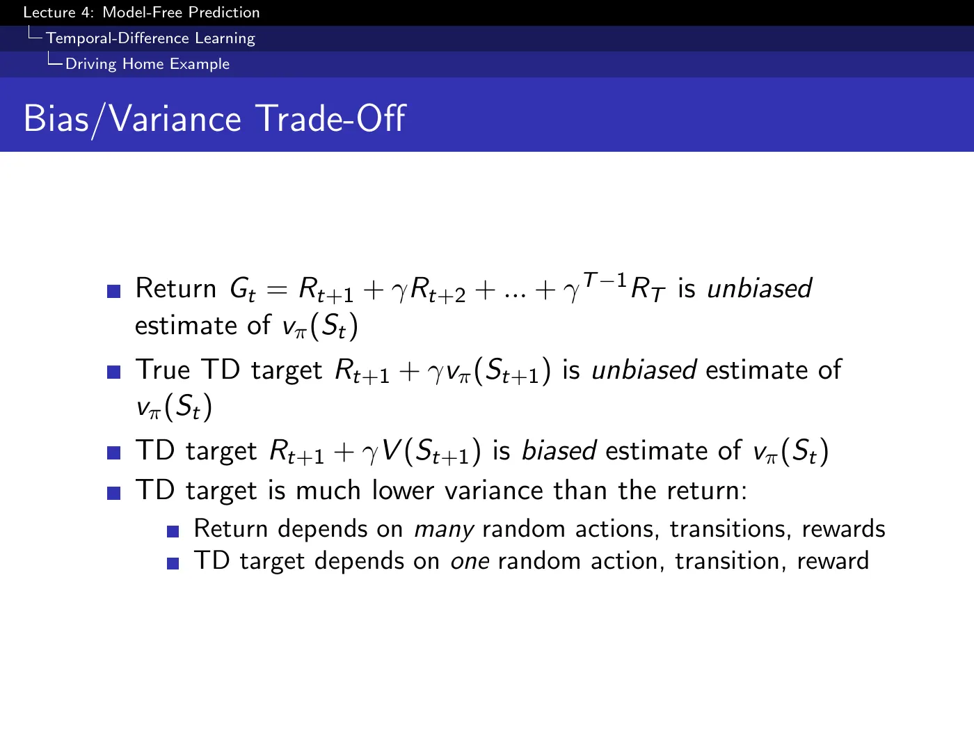
Lecture 4 Model-Free Prediction, slide 17

There are three quantities here and compressing them to two loses the point:

Quantity	Biased?	Why
$G_t$	unbiased	it is a sample of $\mathbb{E}_\pi[G_t]$ , by definition
$R_{t+1}+\gamma v_\pi(S_{t+1})$	unbiased	by the Bellman expectation equation from L2
$R_{t+1}+\gamma V(S_{t+1})$	biased	you substituted your current estimate for $v_\pi$

The bias comes only from the third line. Bootstrapping is not inherently biased; bootstrapping from an estimate that is currently wrong is. As $V\to v_\pi$ the bias vanishes.

The variance argument runs the other way and is purely about how much randomness the target integrates. $G_t$ accumulates noise from every action, transition, and reward for the rest of the episode; the TD target accumulates it from one of each.

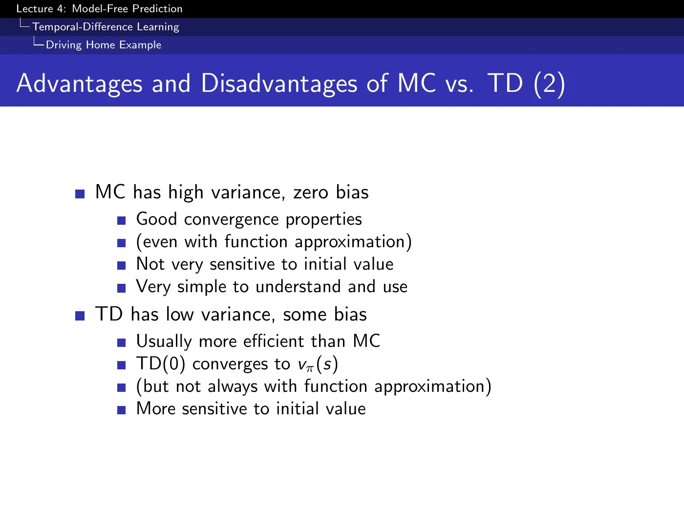
Lecture 4 Model-Free Prediction, slide 18

"TD can learn in continuing environments" is stronger than it looks

The other bullets describe TD being more convenient than MC. This one describes MC being inapplicable. In a non-terminating environment there is no $G_t$ to compute — not a slow one, not a noisy one, none. You can truncate at an arbitrary horizon and accept the error, but there is no Monte-Carlo estimator of the thing you want.
Off-policy learning (L5) creates the same situation for a different reason: you frequently never observe the end of an episode under the target policy.

Is TD's bias just noise in the next state?

No — keep the two separate. Which state you land in is stochastic, and that is variance. The bias is that $V(S_{t+1})\ne v_\pi(S_{t+1})$ — your value function is, at any moment, a fixed and possibly wrong function.
Sharpening it: run TD with the true $v_\pi$ plugged in and the target is unbiased despite the transition still being random. Randomness and wrongness are different failures.

p.19–20 · Random Walk ⏱ 53:06

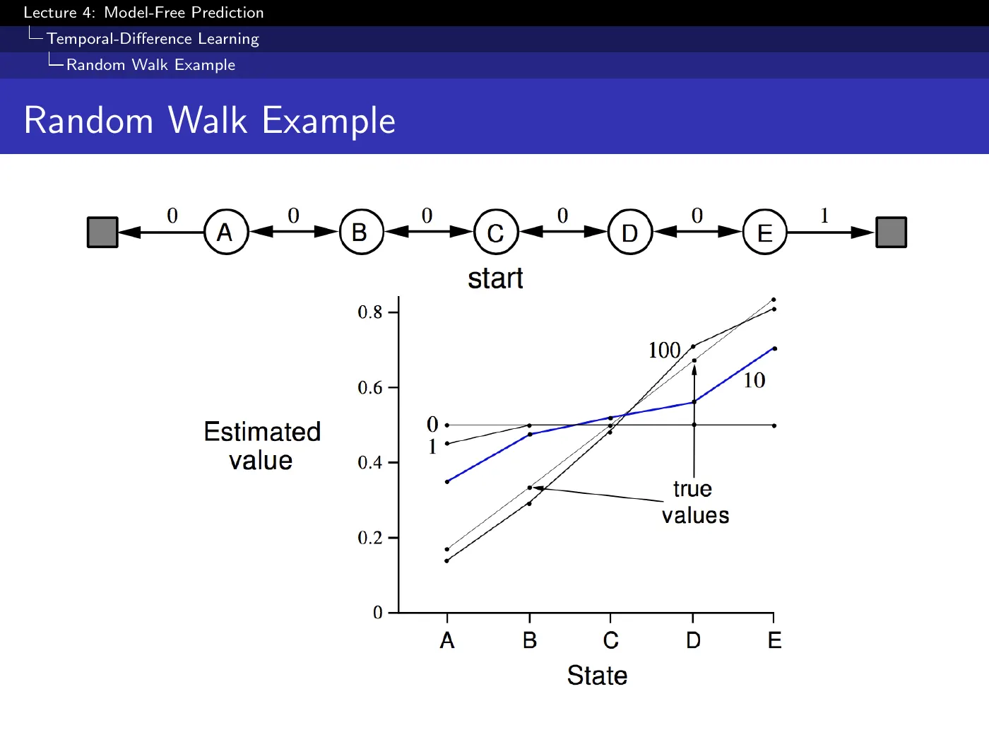
Lecture 4 Model-Free Prediction, slide 19

Five states, uniform random policy, reward $1$ only at the right end. True values are $\tfrac16,\tfrac26,\dots,\tfrac56$ — computable by DP, which is what makes this a clean testbed.

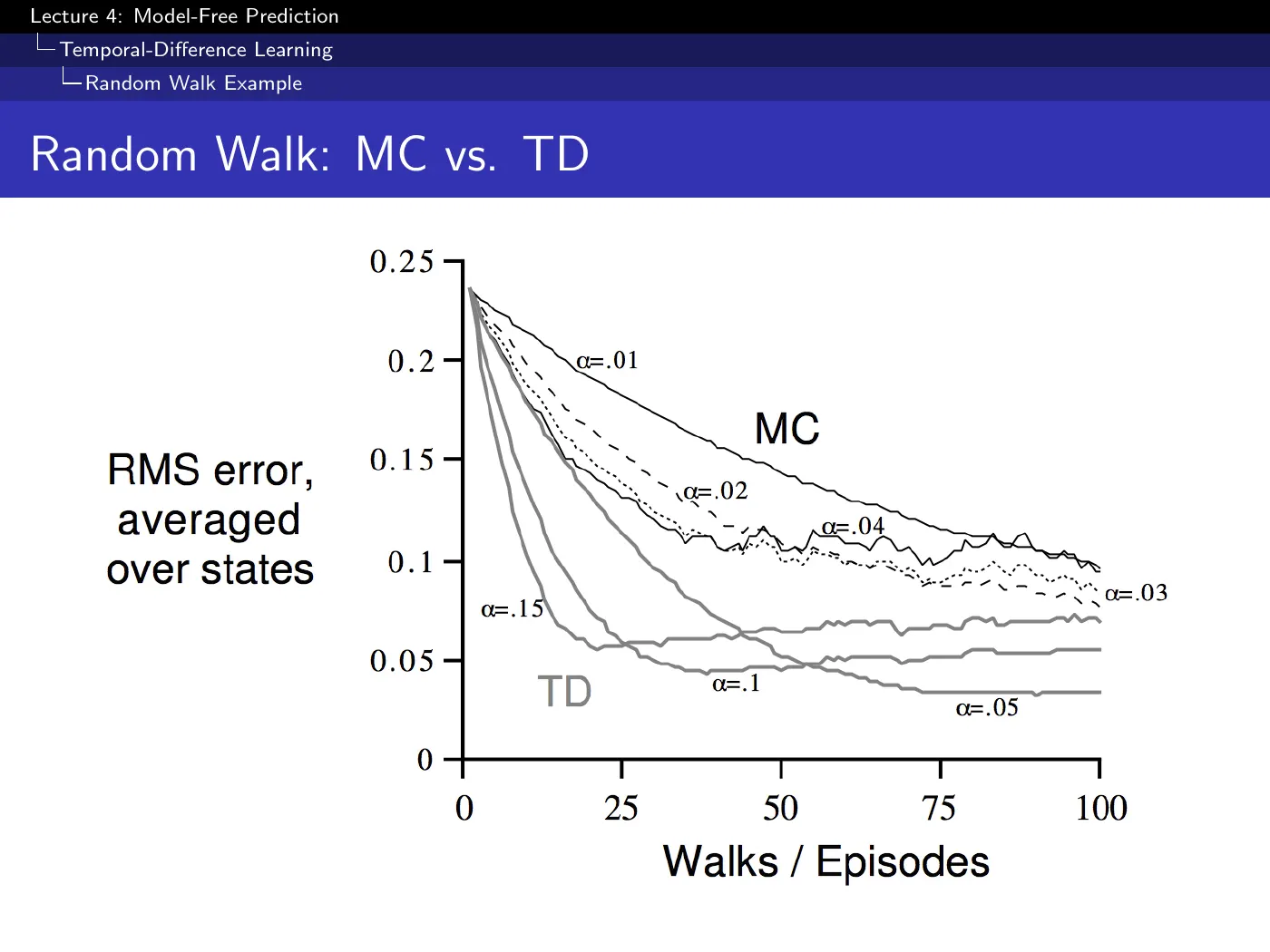
Lecture 4 Model-Free Prediction, slide 20

The y-axis is RMS error averaged over all five states, and TD beats MC at every step size shown.

Some curves drift upward at large α — that is not divergence

With a large fixed step size the estimate cannot settle; it oscillates within a ball whose radius is set by $\alpha$ . It is not diverging and it is not converging.
Exact convergence needs a decaying schedule satisfying the Robbins-Monro conditions — $\sum\alpha_t=\infty$ , $\sum\alpha_t^2<\infty$ — which is the same requirement that reappears for Sarsa in L5. This applies to MC too, and to every gradient method later in the course.

5 · What they converge to

p.21–24 · Batch MC and TD, and the AB Example ⏱ 57:41

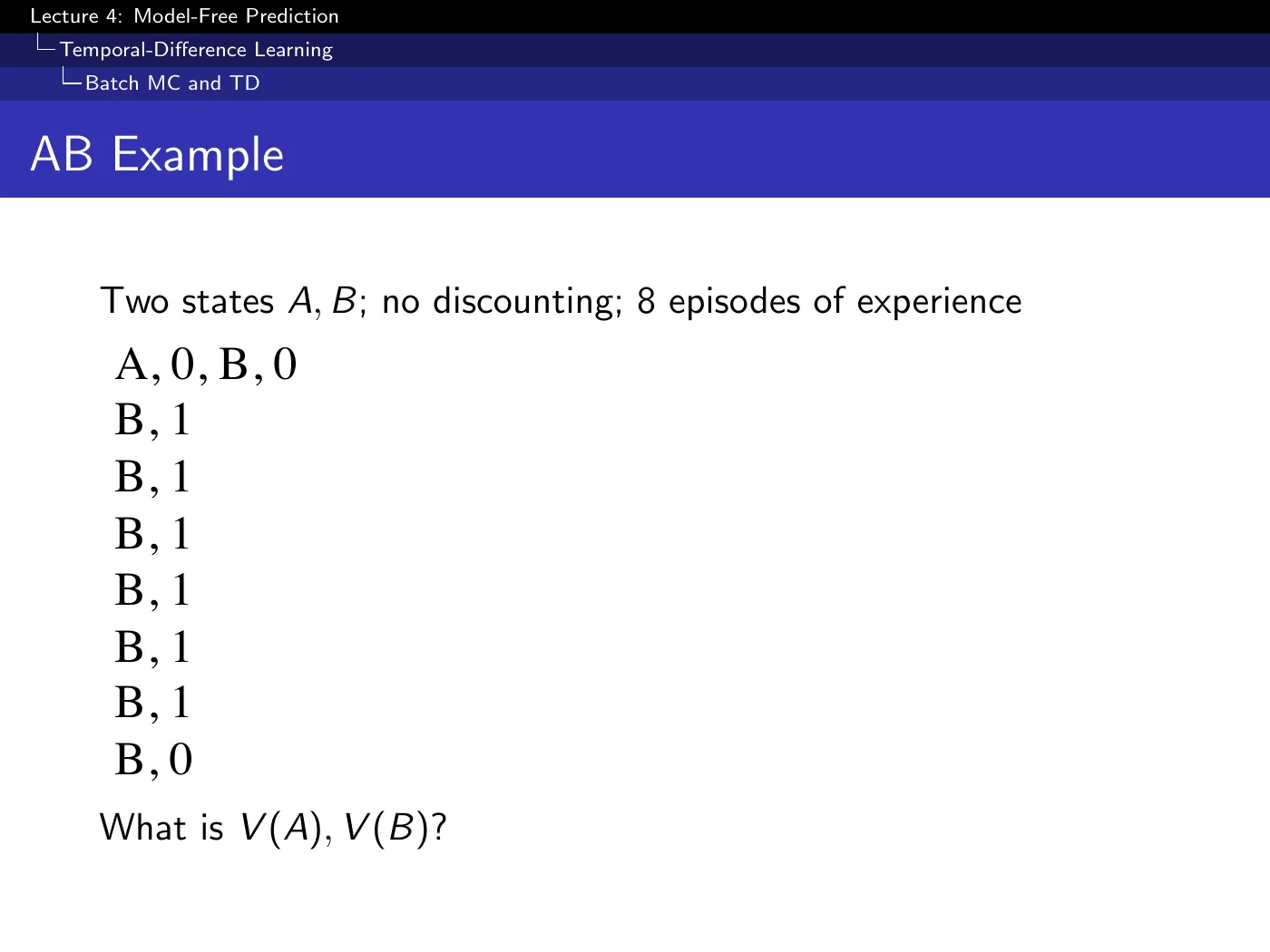
Lecture 4 Model-Free Prediction, slide 22

Eight episodes, two states. $V(B)=6/8=0.75$ is uncontroversial. $V(A)$ splits the room, and both answers are correct — of different questions.

Lecture 4 Model-Free Prediction, slide 24

\text{MC}\;\to\;\arg\min_V\sum_{k=1}^{K}\sum_{t=1}^{T_k}\big(G_t^k-V(s_t^k)\big)^2 \qquad\Longrightarrow\qquad V(A)=0

\text{TD(0)}\;\to\;\text{solution of the MDP }\langle\mathcal{S},\mathcal{A},\hat{\mathcal{P}},\hat{\mathcal{R}},\gamma\rangle \qquad\Longrightarrow\qquad V(A)=0.75

TD is secretly building a model — and this is the single most load-bearing fact in the course

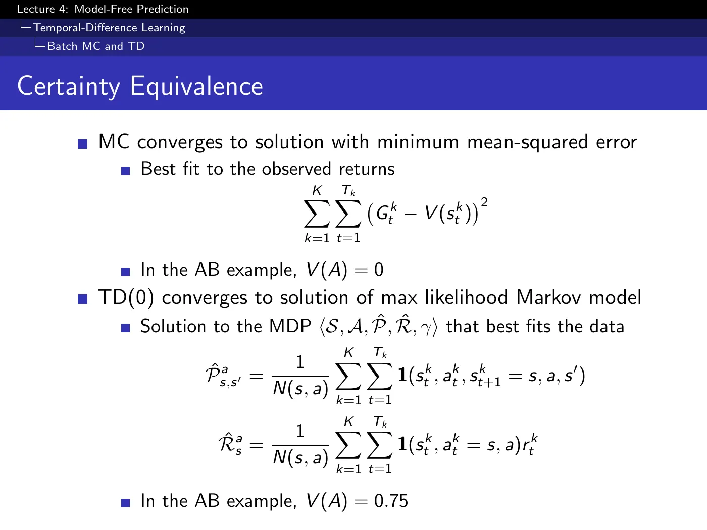
MC fits the returns it literally observed. It saw exactly one episode from $A$ , whose return was $0$ , so $V(A)=0$ . Nothing else enters.
TD behaves as if it first estimated the maximum-likelihood MDP by counting transitions ( $A\to B$ 100% at $r=0$ ; $B\to$ terminal 75% at $r=1$ ) and then solved it. That gives $V(A)=0+V(B)=0.75$ . This is the certainty-equivalence estimate.
The reason $V(A)=0.75$ is better is that TD shares structure across states: what it learned about $B$ from seven episodes transfers to $A$ , because the Markov property says it must.
Follow this thread forward: L8 makes that implicit model explicit and calls it model-based RL, using these same eight episodes → Lecture 8 · Integrating Learning and Planning. Your own worked derivation is in Silver RL Lecture 4 — Question List Q3.

p.25 · Markov Property ⏱ 1:03:49

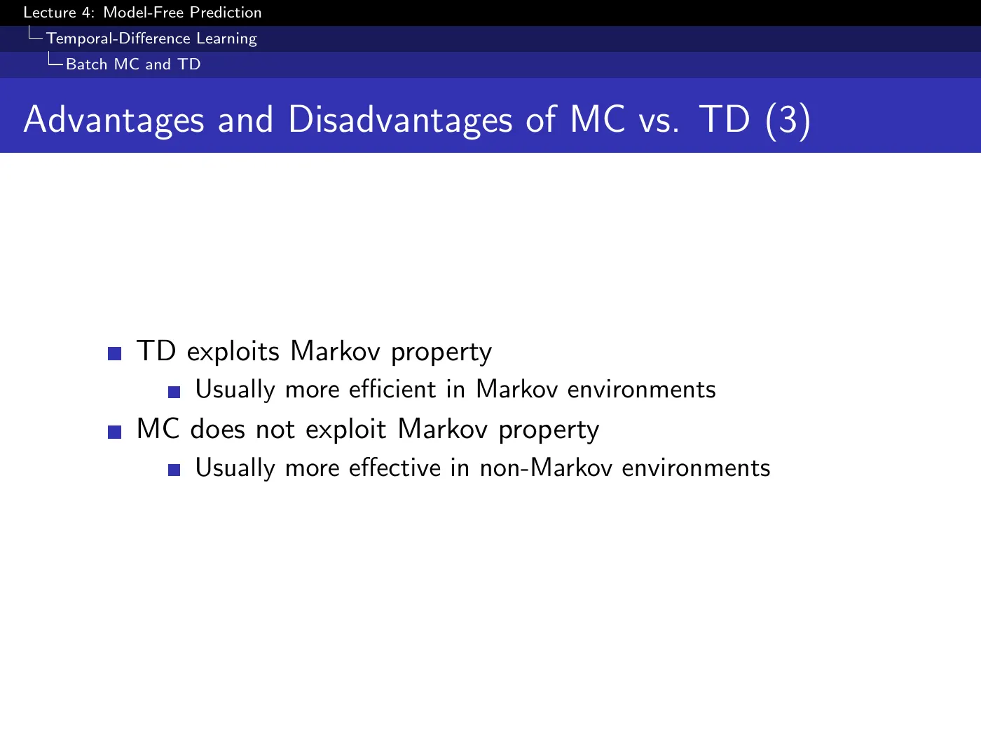
Lecture 4 Model-Free Prediction, slide 25

TD's efficiency and TD's fragility come from the same source: it assumes the state is Markov, and exploits that assumption to share information between states.

In a partially observed environment, is there still an MDP?

Yes, underneath — but you cannot see it. There is an MDP running under the hood; you observe some function of its state, so your representation aliases genuinely different situations together.
MC still does something correct: it consistently estimates the expected return conditioned on the information you gave it. A blind robot's value estimates will be poor, but they will be the right answer to the question its representation can pose.
TD(0) does not. Its whole advantage was exploiting a Markov property that no longer holds, so sharing information between aliased states is now sharing it between states that are not the same.
This is why MC is preferred in non-Markov settings, and it is the L7 aliased-gridworld problem seen from the prediction side.

6 · The unified view

p.26–29 · Backups, Bootstrapping, and Sampling ⏱ 1:06:04

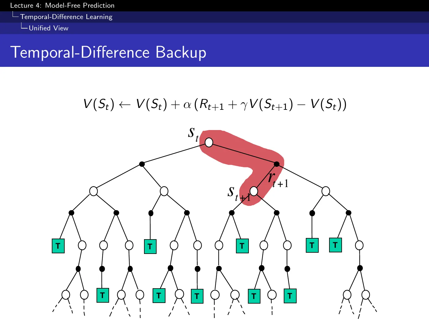
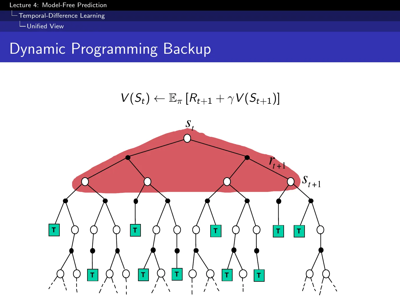
Lecture 4 Model-Free Prediction, slide 27

Lecture 4 Model-Free Prediction, slide 28

Compare the three diagrams as shape: MC is one path all the way down; TD is one path one step deep; DP is every branch one step deep. Depth and width are independent choices, which is exactly what p.29 formalizes.

Lecture 4 Model-Free Prediction, slide 29

Lecture 4 Model-Free Prediction, slide 30

Why does TD update the earlier estimate toward the later one, rather than the reverse?

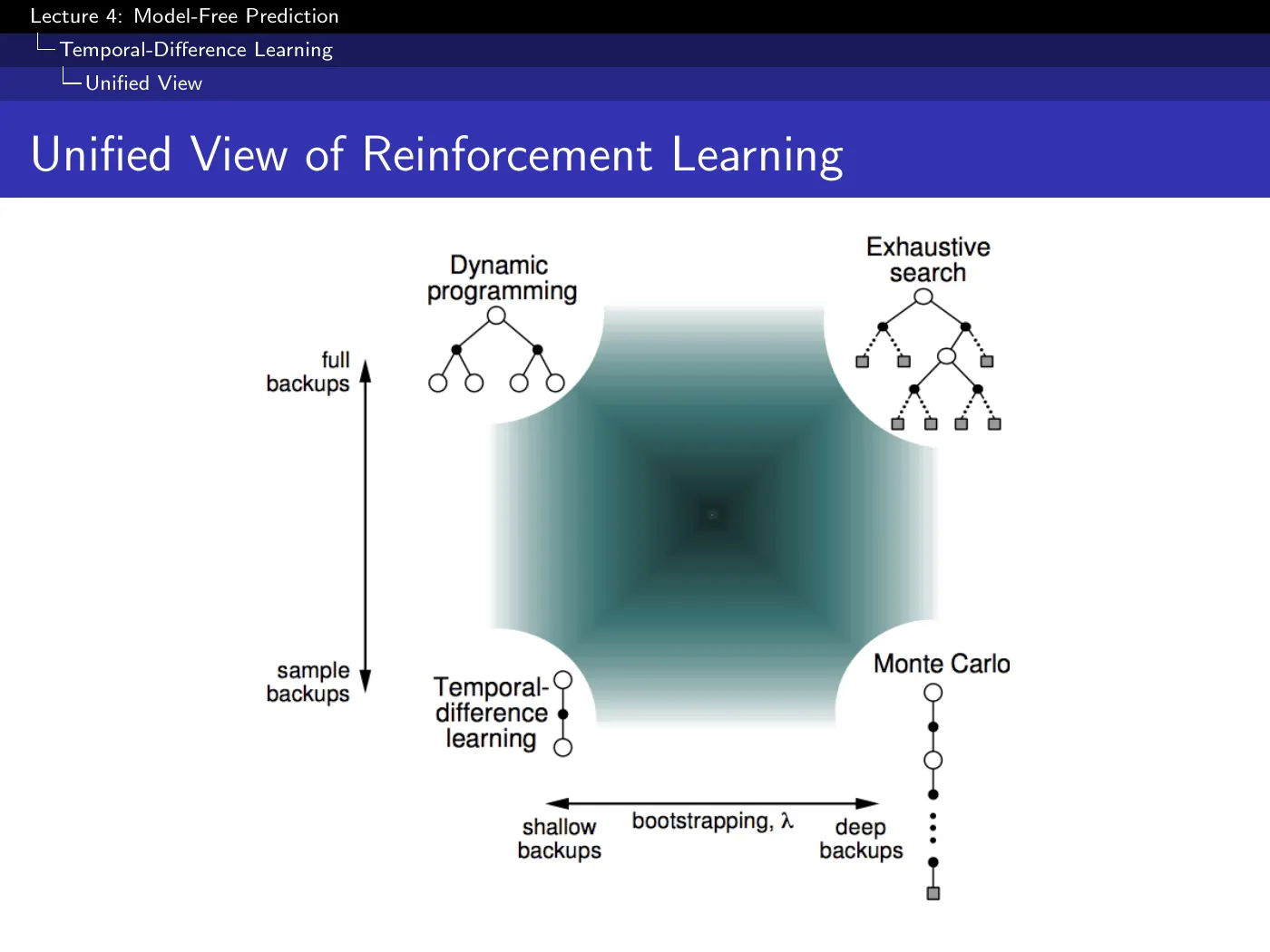
Because the later estimate has seen one step of reality. Between $V(S_t)$ and $V(S_{t+1})$ sits a real sampled reward and a real sampled transition, so the later estimate is grounded in one more piece of the actual environment. Iterate that and you eventually reach a terminal state, where the values are grounded completely.
Reverse the direction and you would be updating an estimate that has already absorbed real information toward one that has not. In a stochastic MDP this converges to the wrong value function — and the same is true of the symmetric variant that tries to minimize the squared TD error over both terms.
Hold onto this. It is the identical question that resurfaces in L6 as "why is the gradient taken only on $\hat v(S,\mathbf{w})$ and not on the TD target?" — with the same answer, and there the consequence is that TD is a semi-gradient method following no objective's gradient.
The lecture promises a specific counterexample MDP and does not give one; see Gaps to close on your own.

If you know the MDP, can you just let Monte-Carlo sample from it?

Yes — and that is a whole later lecture. Silver's answer is "we'll do exactly that in lecture eight or nine."
It becomes sample-based planning: use the model only to generate samples, then run model-free RL on them. Discarding the transition probabilities you know sounds wasteful and is usually a gain, because sampling concentrates effort on outcomes that actually occur instead of expanding every branch → Lecture 8 · Integrating Learning and Planning.

7 · n-step returns

p.31–33 · n-Step Prediction ⏱ 1:16:02

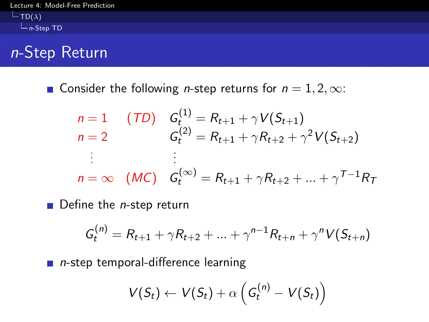
Lecture 4 Model-Free Prediction, slide 32

G_t^{(n)}=R_{t+1}+\gamma R_{t+2}+\dots+\gamma^{n-1}R_{t+n}+\gamma^{n}V(S_{t+n}), \qquad V(S_t)\leftarrow V(S_t)+\alpha\big(G_t^{(n)}-V(S_t)\big)

$n=1$ is TD(0), $n=\infty$ is MC, and everything between is available. Changing $n$ changes how the target is built, never what is being estimated — the quantity is always $v_\pi$ .

Lecture 4 Model-Free Prediction, slide 33

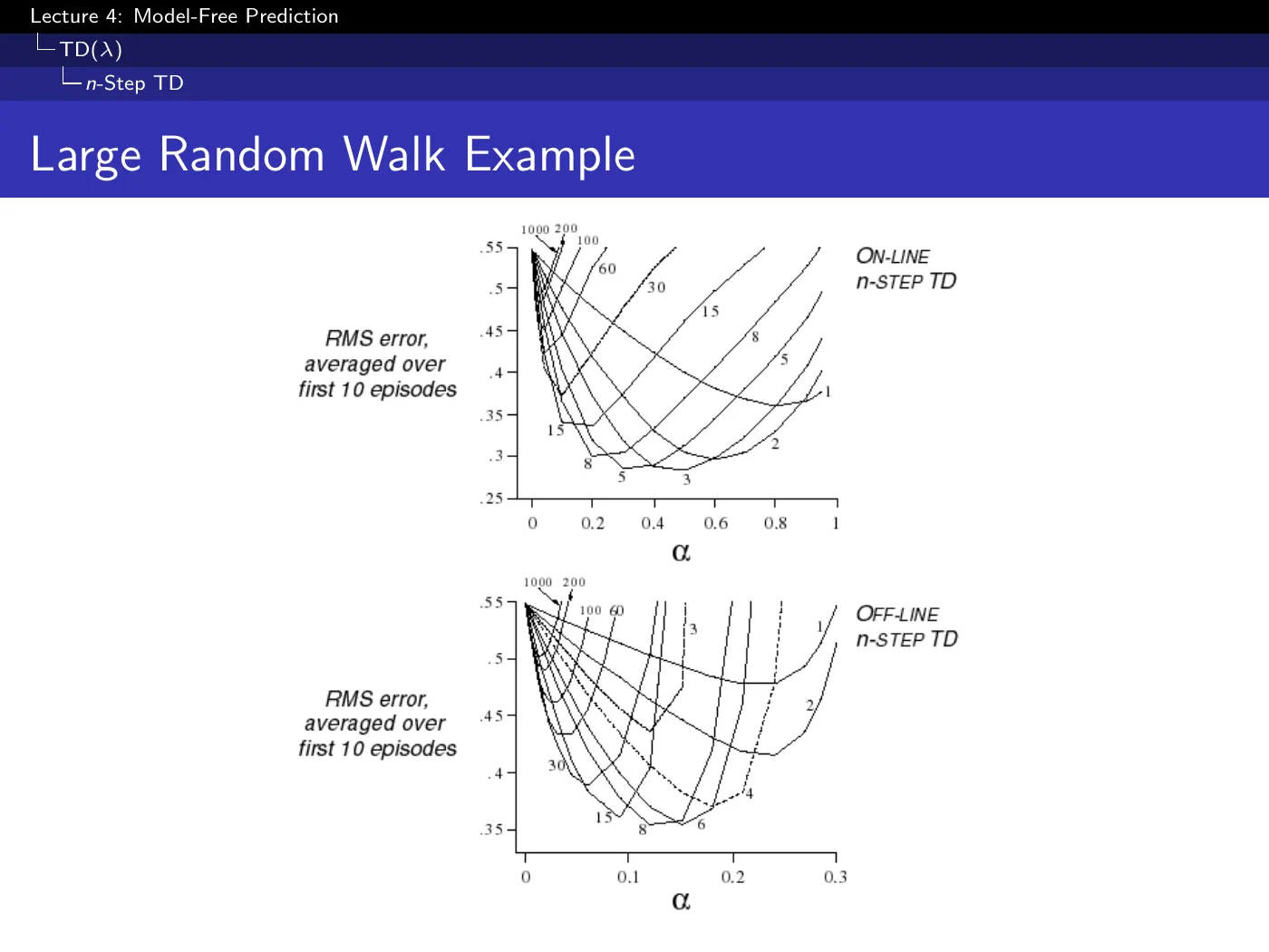
There is a sweet spot around $n=3$ – $5$ , and the reason is mechanical: one $n$ -step update propagates information back $n$ states at once, so credit travels across a long chain far faster than TD(0)'s one-state-per-update crawl.

The sweet spot is the problem, not the answer

The best $n$ moves — it differs between the online and offline panels of the same figure, and it shifts again if you change the length of the random walk. A 100-state walk favors a much larger $n$ than a 19-state one.
So $n$ is a hyperparameter you cannot set without knowing the answer to your problem. That dissatisfaction is precisely what motivates TD( $\lambda$ ): stop choosing an $n$ and average over all of them.

8 · TD-lambda, forward view

p.34–38 · The λ-return ⏱ 1:22:53

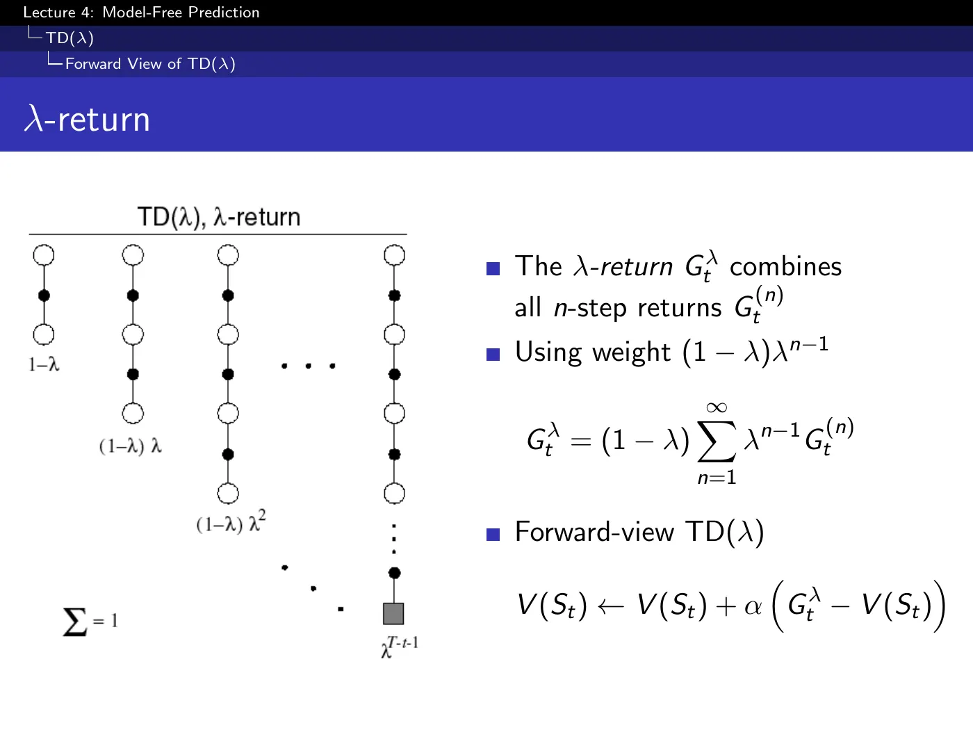
Lecture 4 Model-Free Prediction, slide 35

G_t^{\lambda}=(1-\lambda)\sum_{n=1}^{\infty}\lambda^{n-1}G_t^{(n)}, \qquad V(S_t)\leftarrow V(S_t)+\alpha\big(G_t^{\lambda}-V(S_t)\big)

$(1-\lambda)$ is a normalizer making the weights sum to one — read no meaning into it.

Why geometric weights specifically? Any decaying weighting would blend the n-step returns.

Because geometric weights are memoryless, and that is what makes the algorithm cheap. Under a geometric decay you can compute TD( $\lambda$ ) at essentially the same computational cost as TD(0) — no storing of separate $n$ -step returns, no per- $n$ bookkeeping.
No other weighting scheme buys that. The choice is computational, not statistical, and the backward view on p.41 is where the saving actually materializes.
The property survives a useful generalization: $\lambda$ may vary per time-step and the efficiency still holds, which gives a much broader family than the constant- $\lambda$ version shown.

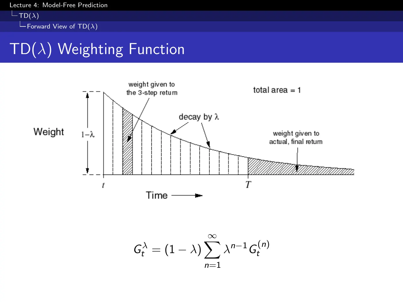
Lecture 4 Model-Free Prediction, slide 36

The last weight is bigger than the one before it, and that is correct

Every weight decays by $\lambda$ until the final one, which spikes. It is not an error.
Think of the terminating episode as an infinite one that enters an absorbing state and collects zero reward forever. Every $n$ -step return beyond termination is then identical, so their weights can be summed and applied once. The spike is that entire remaining tail, collapsed.

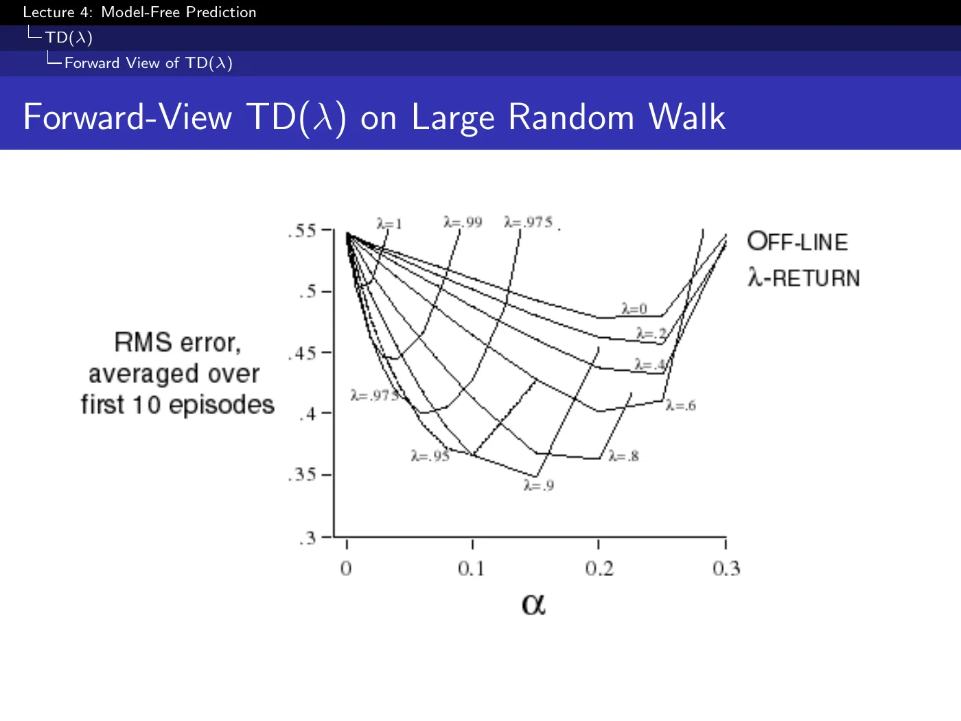
Lecture 4 Model-Free Prediction, slide 38

Compared with the $n$ -step figure, the $\lambda$ curve is far more robust: the best $\lambda$ stays roughly the same as the environment changes, while the best $n$ moved. That robustness is the practical payoff, not raw peak performance.

The defect: $G_t^\lambda$ needs the whole episode, so the forward view is offline — it has inherited exactly the disadvantage TD was introduced to remove.

9 · TD-lambda, backward view

p.39–41 · Eligibility Traces ⏱ 1:30:34

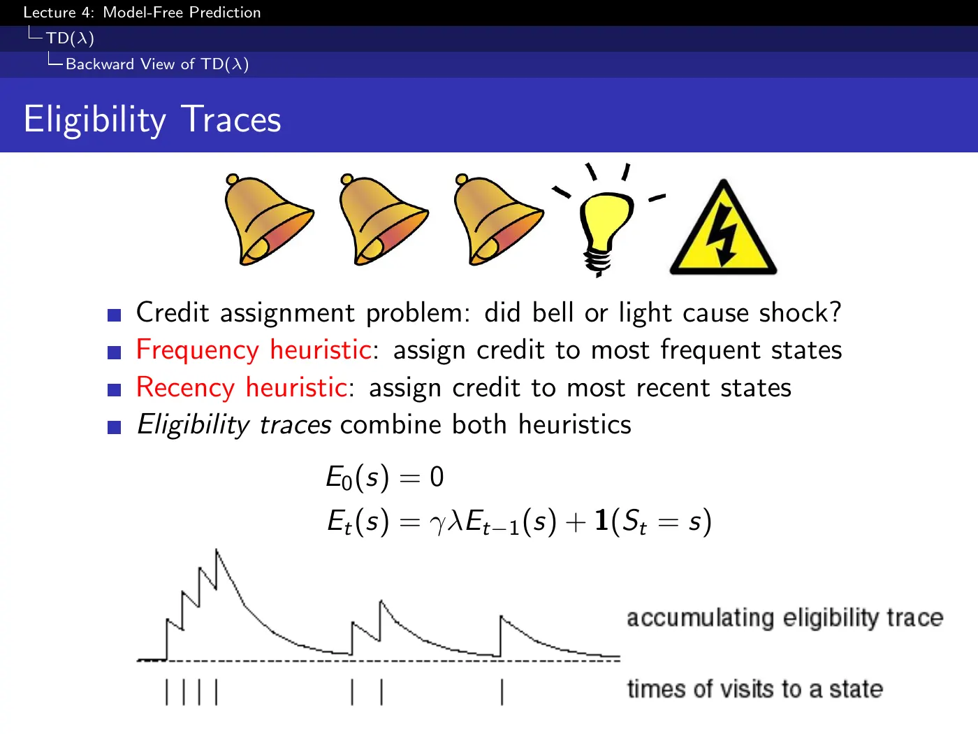
Lecture 4 Model-Free Prediction, slide 40

E_0(s)=0,\qquad E_t(s)=\gamma\lambda E_{t-1}(s)+\mathbf{1}(S_t=s)

The bell rings three times, a light comes on, you are shocked. Which caused it?

Frequency says the bell — it happened most.
Recency says the light — it happened last.

Neither is right alone, and the eligibility trace is simply both at once: increment on visit (frequency), decay by $\gamma\lambda$ otherwise (recency).

Lecture 4 Model-Free Prediction, slide 41

\delta_t=R_{t+1}+\gamma V(S_{t+1})-V(S_t), \qquad V(s)\leftarrow V(s)+\alpha\,\delta_t\,E_t(s)\quad\text{for all }s

Forward view is the definition; backward view is the implementation

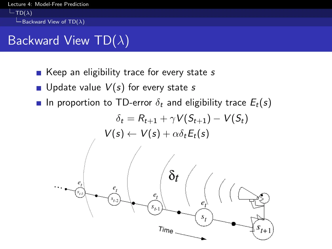
The forward view says what TD( $\lambda$ ) computes — an average over all $n$ -step returns — and cannot be run online. The backward view says how, and reverses the direction of attention: instead of each state looking forward at many returns, each TD error is broadcast backwards to every state, weighted by its eligibility.
Same updates, opposite bookkeeping. That is why one is called forward and the other backward, and it is the reason TD( $\lambda$ ) is usable at all → Forward and Backward Views of TD Lambda.

Note the asymmetry when implementing: increment the trace for the one state you visited, but decay and update every state.

p.42–43 · The Two Ends, and the Equivalence Theorem ⏱ 1:33:36

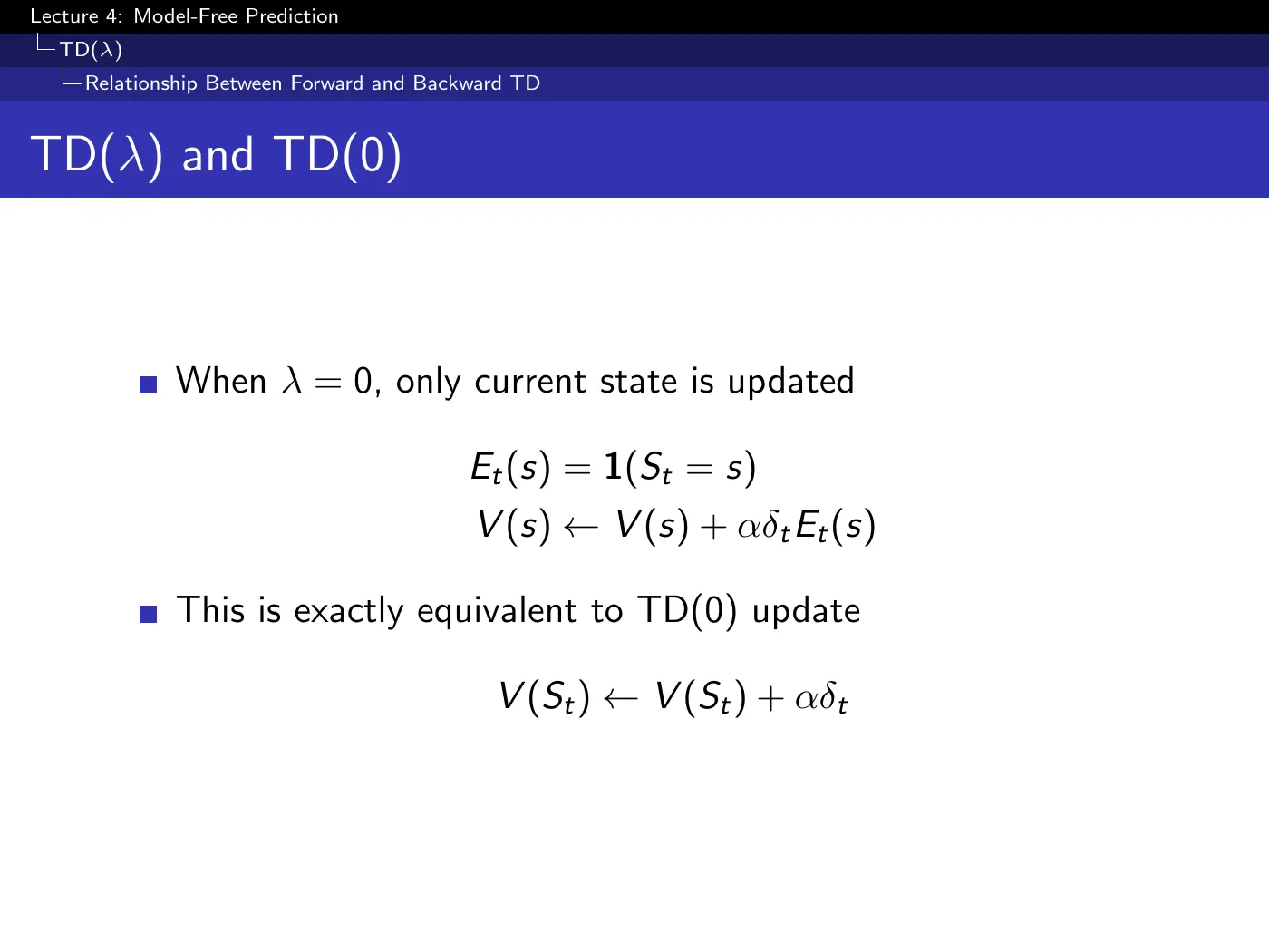
Lecture 4 Model-Free Prediction, slide 42

$\lambda=0$ makes the trace $\mathbf{1}(S_t=s)$ — nonzero only at the current state — so the update collapses to exactly TD(0). That is where the name comes from.

Lecture 4 Model-Free Prediction, slide 43

\sum_{t=1}^{T}\alpha\,\delta_t E_t(s)=\sum_{t=1}^{T}\alpha\big(G_t^\lambda-V(S_t)\big)\mathbf{1}(S_t=s)

Read the theorem's conditions, not just its conclusion

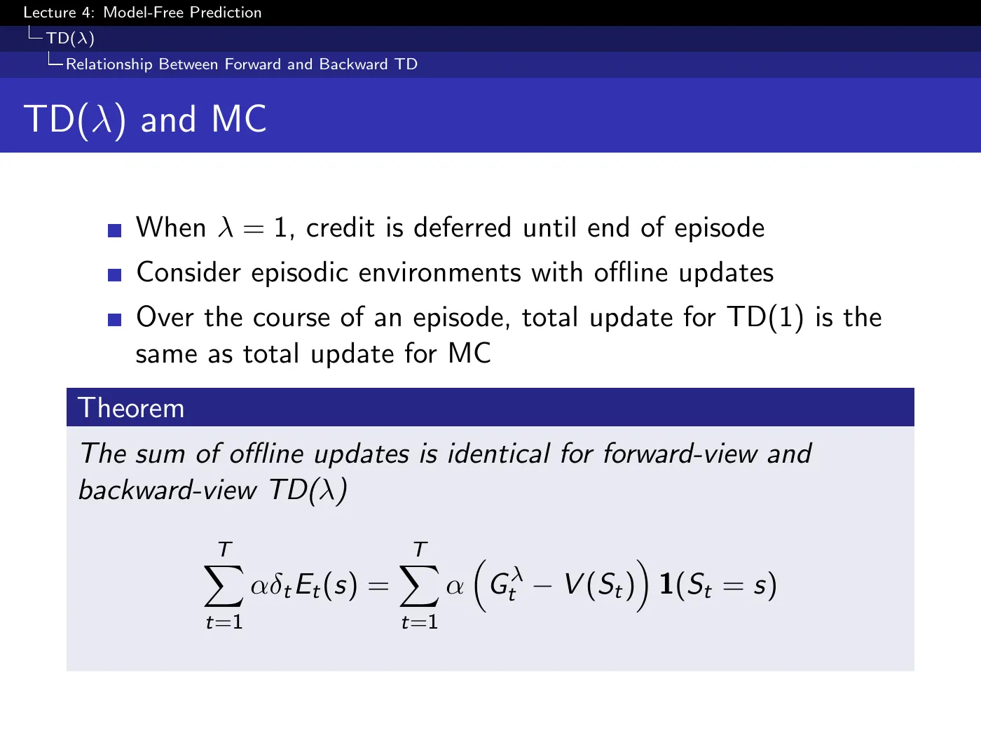
It is an equality of summed offline updates — accumulate within the episode, apply in a batch at the end. Under online updating, forward and backward TD( $\lambda$ ) are not identical (p.50), because each changes $V$ as it goes and so changes the other's inputs.
Exact equivalence under online updates was only achieved later, with a modified trace (Sutton & von Seijen, ICML 2014). p.51's summary table is the precise bookkeeping of which cells are $=$ and which are $\ne$ .

Study checklist

Answer these without the notes before moving on to L5. Each item links back to where it is worked out; open the toggle only after you have tried.

1. What single question organizes this entire lecture?
→ p.31–33 · n-Step Prediction ⏱ 1:16:02

Answer

How far into the real trajectory do you look before substituting your own guess for the rest? MC looks all the way ( $G_t$ ), TD(0) looks one step ( $R_{t+1}+\gamma V(S_{t+1})$ ), $n$ -step looks $n$ , TD( $\lambda$ ) blends every $n$ geometrically.
All of them slot a different target into the same template: $\text{new}\leftarrow\text{old}+\alpha(\text{target}-\text{old})$ .

2. Why is MC's cost independent of the size of the state space?
→ p.6–7 · First-Visit and Every-Visit MC ⏱ 9:01

Answer

By the central limit theorem the error variance shrinks like $1/N(s)$ , where $N(s)$ counts visits to that state — nothing in the rate refers to $|\mathcal{S}|$ .
DP swept every state every iteration; MC pays only for states it visits, in proportion to visitation frequency. That is the structural reason sampling escapes the curse of dimensionality.
Corollary from blackjack: your bottleneck is rare states. The usable-ace surface is still noisy at 10,000 episodes and needs ~500,000, because those states occur rarely — not because there are many of them.

3. Give the three quantities in the bias discussion and say exactly where the bias enters.
→ p.16–18 · MC versus TD ⏱ 44:45

Answer

$G_t$ — unbiased, it is by definition a sample of $\mathbb{E}_\pi[G_t]$ .
$R_{t+1}+\gamma v_\pi(S_{t+1})$ — unbiased, by the Bellman expectation equation.
$R_{t+1}+\gamma V(S_{t+1})$ — biased, because you substituted your current estimate for $v_\pi$ .
Bootstrapping is not inherently biased; bootstrapping from a currently-wrong estimate is, and the bias vanishes as $V\to v_\pi$ . Variance runs the opposite way: $G_t$ accumulates noise over the whole episode, the TD target over one step.

4. Why can TD learn from a near-miss when MC cannot?
→ p.12–13 · TD(0) ⏱ 34:07

Answer

A car nearly hits you and swerves away. No crash happens, so the return carries no penalty and MC has nothing to learn from.
TD sees the estimate jump from "fine" to "about to die" in one step — a large TD error — and updates the earlier state immediately. A change in prediction is itself a learning signal, so you need not experience the outcome to learn from the situation.

5. In the AB example, why is $V(A)=0$ and $V(A)=0.75$ both right, and which is TD's?
→ p.21–24 · Batch MC and TD, and the AB Example ⏱ 57:41

Answer

MC → $V(A)=0$ : it minimizes squared error against the returns actually observed, and the single episode from $A$ returned $0$ .
TD → $V(A)=0.75$ : it converges to the solution of the maximum-likelihood MDP built by counting transitions ( $A\to B$ at 100%, $r=0$ ; $B\to$ terminal 75% at $r=1$ ), giving $V(A)=0+V(B)$ . This is the certainty-equivalence estimate.
TD wins here by sharing structure: what seven episodes taught it about $B$ transfers to $A$ because the Markov property says it must. L8 makes that implicit model explicit.

6. Why is TD more efficient in Markov environments and worse in non-Markov ones?
→ p.25 · Markov Property ⏱ 1:03:49

Answer

Both follow from the same fact: TD assumes the state is Markov and exploits it to share information between states (see the AB example).
Under partial observability that assumption fails — your representation aliases genuinely different situations — so the sharing is now between states that are not the same, and TD(0) misbehaves.
MC stays consistent: it estimates the expected return conditioned on the representation you gave it. Poor if the representation is poor, but the right answer to the question that representation can pose.

7. State the two axes of the unified view and place all four methods.
→ p.26–29 · Backups, Bootstrapping, and Sampling ⏱ 1:06:04

Answer

Bootstrapping (does the target contain your own estimate) and sampling (or expand the full expectation) — two independent questions.

	full-width	sample
no bootstrap	exhaustive tree search	Monte-Carlo
bootstrap	dynamic programming	TD

DP and MC are not opposites — they differ on both axes. TD takes one property from each.

8. Why does TD update the earlier estimate toward the later one rather than the reverse?
→ p.26–29 · Backups, Bootstrapping, and Sampling ⏱ 1:06:04

Answer

Because the later estimate has seen one step of reality — a real sampled reward and a real sampled transition sit between them, so it is grounded in one more piece of the environment. Iterate and you reach terminal states, which are fully grounded.
Reversing it updates an estimate that absorbed real information toward one that did not, and in stochastic MDPs it converges to the wrong value function.
Same question, same answer, bigger consequence in L6: this is why TD is a semi-gradient method that follows no objective's gradient.

9. What does changing $n$ change, and why is the sweet spot unsatisfying?
→ p.31–33 · n-Step Prediction ⏱ 1:16:02

Answer

It changes how the target is built, never what is being estimated — the quantity is always $v_\pi$ . Larger $n$ propagates credit back $n$ states per update instead of one.
The sweet spot ( $n\approx 3$ – $5$ here) moves: it differs between online and offline updating in the same figure, and shifts again with the length of the walk. So $n$ cannot be set without already knowing your problem — which is what motivates averaging over all $n$ .

10. Why geometric weights in the λ-return, and why is the final weight larger?
→ p.34–38 · The λ-return ⏱ 1:22:53

Answer

Geometric because it is memoryless, which lets TD( $\lambda$ ) run at essentially the same computational cost as TD(0) — no storing per- $n$ returns. The reason is computational, not statistical, and the saving materializes in the backward view. ( $\lambda$ may even vary per step and the property survives.)
The final weight spikes because a terminating episode is an infinite one sitting in an absorbing state at zero reward: every $n$ -step return past termination is identical, so their weights collapse into a single update.

11. What do eligibility traces solve, and how do the two views relate?
→ p.39–41 · Eligibility Traces ⏱ 1:30:34

Answer

Credit assignment. Bell rings three times, light comes on, shock — frequency blames the bell, recency blames the light, and $E_t(s)=\gamma\lambda E_{t-1}(s)+\mathbf{1}(S_t=s)$ does both (increment on visit, decay otherwise).
Forward view = definition (average over all $n$ -step returns, requires the full episode). Backward view = implementation (broadcast each TD error backwards to all states, weighted by eligibility). Same updates, opposite bookkeeping; only the backward one runs online.
Implementation asymmetry: increment the trace for the one state visited, decay and update every state.

12. State the forward/backward equivalence theorem's conditions.
→ p.42–43 · The Two Ends, and the Equivalence Theorem ⏱ 1:33:36

Answer

$\sum_t\alpha\delta_t E_t(s)=\sum_t\alpha(G_t^\lambda-V(S_t))\mathbf{1}(S_t=s)$ — equality of summed offline updates, accumulated within the episode and applied in batch at the end.
Under online updating they are not identical, because each view changes $V$ as it goes and therefore changes the other's inputs. Exact online equivalence needed a modified trace (Sutton & von Seijen, ICML 2014).
$\lambda=0$ makes the trace $\mathbf{1}(S_t=s)$ and the update collapses to exactly TD(0).

Gaps to close on your own

Slides p.44–48 and p.51 are deferred to self-study

The lecture states the equivalence theorem and explicitly leaves the proofs as notes to read afterwards, running out of time before the summary table.

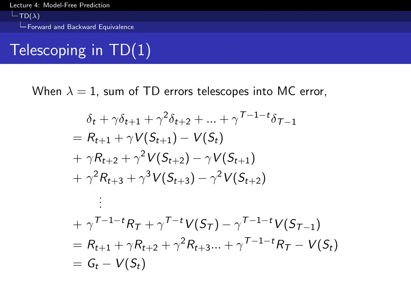
Lecture 4 Model-Free Prediction, slide 45

p.44–45 are the $\lambda=1$ case: the TD(1) trace is $\gamma^{t-k}$ after a visit at time $k$ , and the sum of discounted TD errors telescopes into $G_k-V(S_k)$ — every intermediate $\gamma^{j}V(S_j)$ term cancels against its neighbor, leaving only real rewards and the initial estimate. That single cancellation is why TD(1) equals every-visit MC.

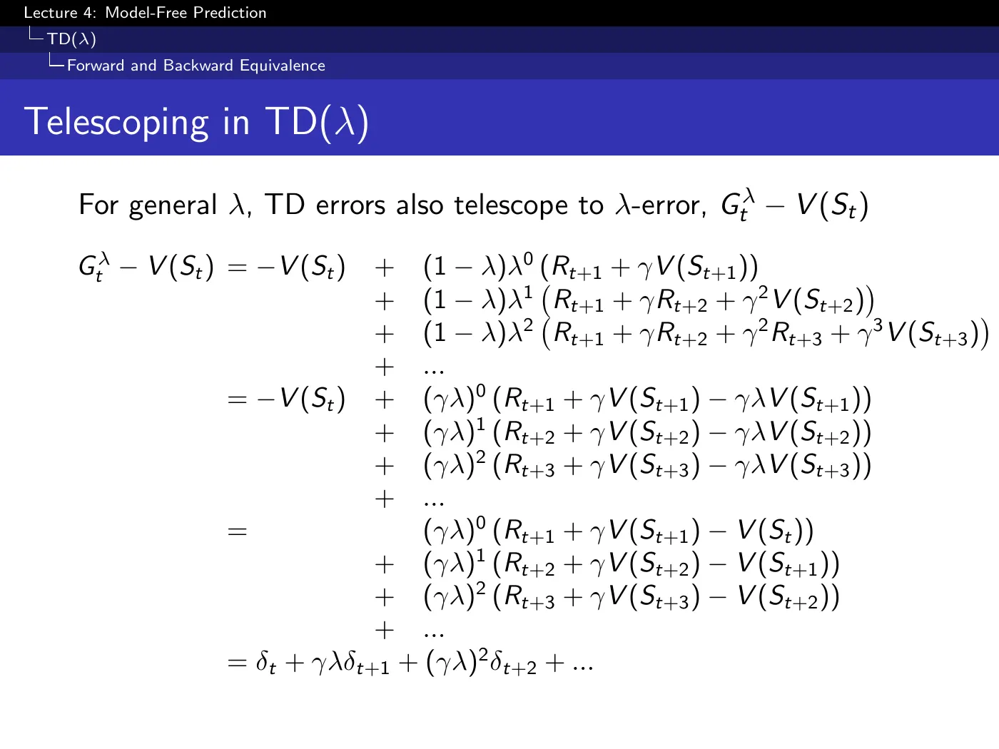
Lecture 4 Model-Free Prediction, slide 47

p.47–48 generalize the same telescoping to arbitrary $\lambda$ , with $(\gamma\lambda)^{t-k}$ in place of $\gamma^{t-k}$ .

Lecture 4 Model-Free Prediction, slide 51

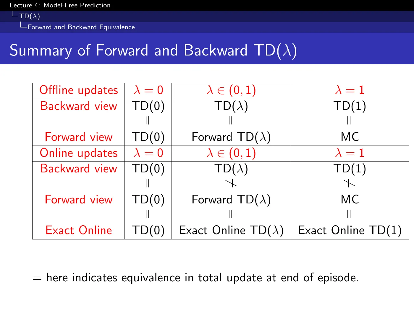
p.51 is worth reading even without the proofs — it is the exact map of which cells are $=$ and which are $\ne$ across offline/online and $\lambda\in\{0,(0,1),1\}$ .

The counterexample for reversed TD updates. The lecture asserts that updating backwards gives the wrong answer in stochastic MDPs and promises a specific small MDP demonstrating it, which it never provides. Worth constructing yourself — it is the concrete form of the semi-gradient argument in L6.
The TD(0) convergence proof. Stated as true for table lookup and attributed to Peter Dayan; not proved. The function-approximation caveat is deferred to L6, where it becomes the whole convergence section.
First-visit versus every-visit. Both are declared consistent and the lecture declines to rank them, noting evidence for each depending on domain. The connection to accumulating versus replacing traces is mentioned and not developed.
Exact online TD( $\lambda$ ). Named on p.50 with a citation (Sutton & von Seijen, ICML 2014) and no mechanism. If you implement TD( $\lambda$ ) online and want the forward-view guarantee, this is the gap.

Language notes

Phrasings worth stealing for your own technical writing and talks:

Expression	Use
update a guess towards a guess	naming bootstrapping in five words
you can't back up death	why an outcome-only learner misses near-misses
it doesn't feed off itself	a method whose errors do not compound through self-reference
grounded by the actual outcome	an estimate ultimately anchored to observed reality
the noise multiplies out over the trajectory	variance accumulating along a sequence
it's a bit unsatisfactory	conceding a method works but needs a hyperparameter you cannot set
the best of all n	motivating an average over a family instead of choosing one member
a sweet spot in between	an interior optimum between two extremes
credit assignment	apportioning responsibility for a delayed outcome
forward view provides theory, backward view provides mechanism	separating what a method computes from how it runs

The one idea

Contents

1 · Monte-Carlo policy evaluation

p.3–5 · Model-Free Prediction ⏱ 2:15

p.6–7 · First-Visit and Every-Visit MC ⏱ 9:01

p.8–9 · Blackjack ⏱ 16:37

2 · Incremental updates

p.10–11 · Incremental Mean and Incremental MC ⏱ 26:29

3 · Temporal-difference learning

p.12–13 · TD(0) ⏱ 34:07

p.14–15 · Driving Home ⏱ 39:27

4 · Bias and variance

p.16–18 · MC versus TD ⏱ 44:45

p.19–20 · Random Walk ⏱ 53:06

5 · What they converge to

p.21–24 · Batch MC and TD, and the AB Example ⏱ 57:41

p.25 · Markov Property ⏱ 1:03:49

6 · The unified view

p.26–29 · Backups, Bootstrapping, and Sampling ⏱ 1:06:04

7 · n-step returns

p.31–33 · n-Step Prediction ⏱ 1:16:02

8 · TD-lambda, forward view

p.34–38 · The λ-return ⏱ 1:22:53

9 · TD-lambda, backward view

p.39–41 · Eligibility Traces ⏱ 1:30:34

p.42–43 · The Two Ends, and the Equivalence Theorem ⏱ 1:33:36

Study checklist

Gaps to close on your own

Language notes