Lecture 9 · Exploration and Exploitation

Slides: David Silver - RL Course (UCL 2015) · Previous: Lecture 8 · Integrating Learning and Planning · Next: Lecture 10 · Classic Games

First pass: read The one idea and the slide-group headings. Use the prose when an equation, condition, or figure needs explanation; leave Gaps to close for review.

The one idea

Every previous lecture reached for $\epsilon$ -greedy and moved on. L9 finally asks whether that was any good. A fixed $\epsilon$ gives linear regret, while a suitable decaying schedule can achieve logarithmic regret. The difficulty is choosing that schedule without already knowing the reward gaps.

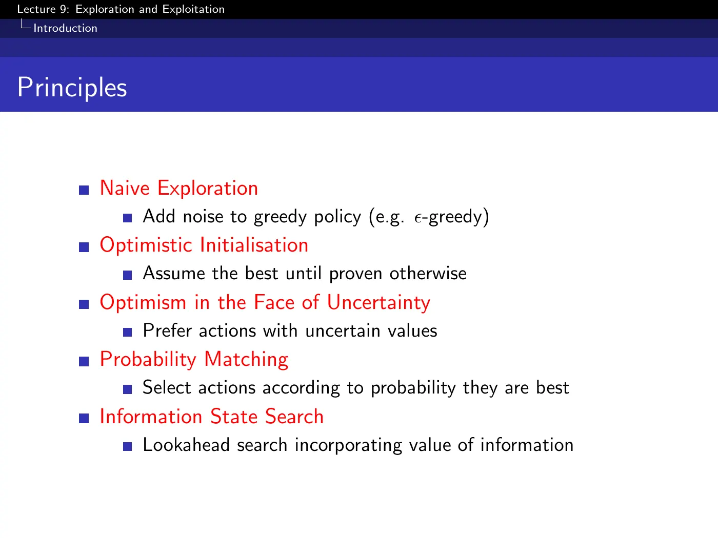
The whole lecture is one small matrix — a principle, applied in a setting:

Principle	Bandit	Contextual bandit	MDP
Naive / random exploration	$\epsilon$ -greedy, softmax	—	$\epsilon$ -greedy
Optimistic initialization	optimistic $\hat Q$	—	optimistic $\hat Q$ / optimistic model (RMax)
Optimism in the face of uncertainty	UCB1, Bayesian UCB	LinUCB	UCB on $Q$
Probability matching	Thompson sampling	—	Thompson sampling on MDPs
Information state search	Gittins, Bayes-adaptive	—	Bayes-adaptive MDP

Every row is developed in the leftmost column and then transplanted rightward. The final slide says exactly this, so the bandit section is not a warm-up — it is the lecture.

The measuring stick is regret, and it turns the whole subject into one question

Instead of "how much reward did I get", ask "how much did I lose against an oracle who knew the best arm from the start". Total regret decomposes as $L_t=\sum_a\mathbb{E}[N_t(a)]\,\Delta_a$ — counts times gaps.
That reframing makes the goal concrete: pull high-gap arms few times. And it exposes the central obstacle in one line, which the slide states almost in passing: you do not know the gaps. Every algorithm in this lecture is a different way of acting well without them.

The classification that organizes everything — linear vs sublinear regret

If you explore forever at a fixed rate, you pay a constant regret every step → linear. If you never explore, you can lock onto a wrong arm forever → also linear. Both extremes fail the same way and for opposite reasons.
Sublinear regret requires an algorithm whose rate of mistakes falls over time. That rules out pure greedy in the worst case, fixed- $\epsilon$ exploration, and one-shot optimistic initialization as general guarantees. Decaying $\epsilon$ -greedy, UCB, and Thompson sampling are different ways to make exploration adapt with evidence.

There is a whole axis of exploration that appears on no slide

The lecture spends three minutes (⏱ 8:22) on a distinction it calls fundamental and under-discussed, and then never puts it on a slide: where you explore.

State-action space exploration — $\epsilon$ -greedy and everything else in this lecture. You track what you have tried where, and use that to explore systematically.
Parameter space exploration — perturb the policy parameters and run the resulting policy for a while. This is what you do to an AIBO gait — L7 p.14.

Parameter exploration buys consistency: you commit to a coherent alternative behavior and see how it does, instead of re-randomizing every step and executing a random walk. That matters in robotics, where per-step noise gets you nowhere.
What it gives up is everything: it has no notion of state or action coverage, cannot recognize a state it has visited, and is really global optimization in parameter space presented as exploration. Nothing else in this lecture applies to it.

1 · The dilemma and the yardstick
2 · Why the naive methods fail
3 · The lower bound
4 · Optimism in the face of uncertainty
5 · Bayesian bandits and probability matching
6 · Information state search
7 · Contextual bandits
8 · Back to MDPs
Study checklist
Gaps to close on your own
Language notes

1 · The dilemma and the yardstick

p.3–5 · The Dilemma and the Principles ⏱ 2:18

Lecture 9 Exploration and Exploitation, slide 5

The reason this problem exists at all is worth stating once: you are learning online, and your actions determine the data you see. In supervised learning someone hands you a dataset and you optimize over it. Here there is no dataset until you go and generate it, and a greedy learner generates a dataset that confirms whatever it already believes.

The video reorganizes these five principles into three families, which is the more useful grouping to carry:

Family	Members	Character
Random exploration	$\epsilon$ -greedy, softmax, Gaussian noise	myopic — never looks at what it knows
Optimism in the face of uncertainty	optimistic initialization, UCB, Thompson sampling	uses a measure of what it does not know
Information state search	Gittins, Bayes-adaptive RL	treats knowledge itself as state; theoretically correct, computationally intractable

The three are ordered by how much they exploit accumulated knowledge, and correspondingly by cost.

p.6–8 · The Multi-Armed Bandit and Regret ⏱ 12:09

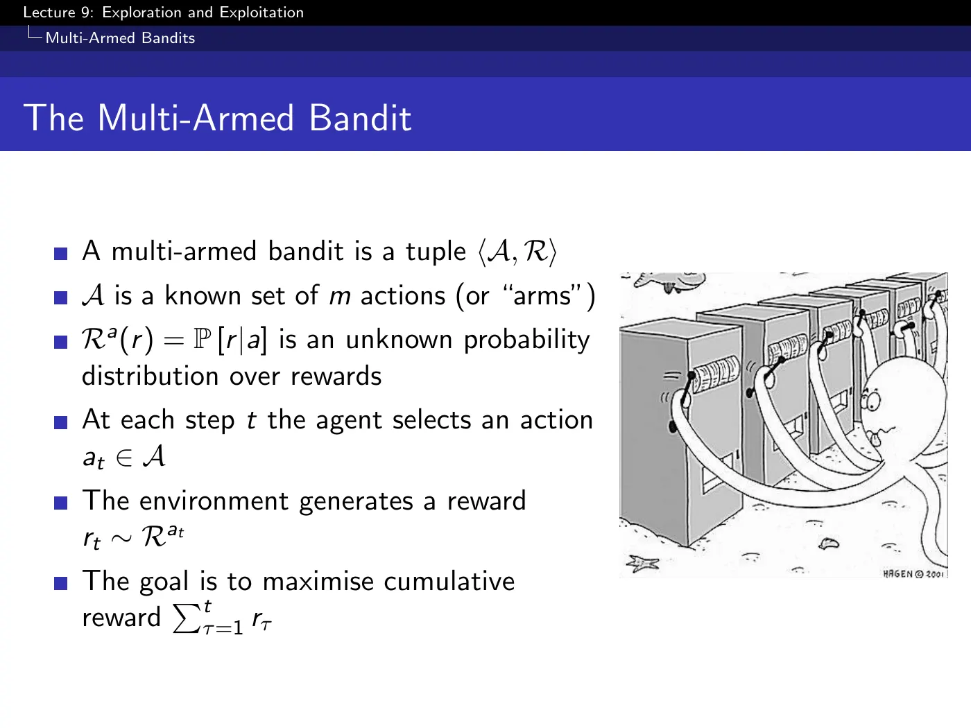
Lecture 9 Exploration and Exploitation, slide 6

A bandit is an MDP with the state space and the transition function deleted — $\langle\mathcal{A},\mathcal{R}\rangle$ , one step, one reward, done. Strip away everything else and what remains is exploration in its purest form, which is why the lecture spends most of its time here.

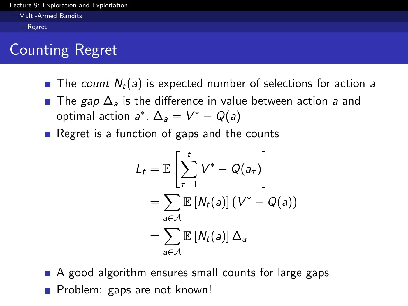
Lecture 9 Exploration and Exploitation, slide 8

L_t=\mathbb{E}\left[\sum_{\tau=1}^{t}V^*-Q(a_\tau)\right]=\sum_{a\in\mathcal{A}}\mathbb{E}[N_t(a)]\,\big(V^*-Q(a)\big)=\sum_{a\in\mathcal{A}}\mathbb{E}[N_t(a)]\,\Delta_a

The rewrite from a sum over time to a sum over actions is the move that makes the rest of the lecture possible. Once regret is counts × gaps, "explore well" becomes the concrete instruction keep counts small where gaps are large.

Two things the slide does not say:

Why regret rather than raw reward. Regret compares an algorithm with an oracle on the same problem, separating learning loss from the problem's baseline reward. It is not invariant to reward scaling: multiply all rewards by $c$ and regret also scales by $c$ .
The gaps are defined against $V^*$ , which is exactly what you are trying to find. The decomposition is a diagnostic, not an algorithm. The final bullet — "Problem: gaps are not known!" — is the entire remaining lecture.

2 · Why the naive methods fail

p.9 · Linear or Sublinear Regret ⏱ 21:17

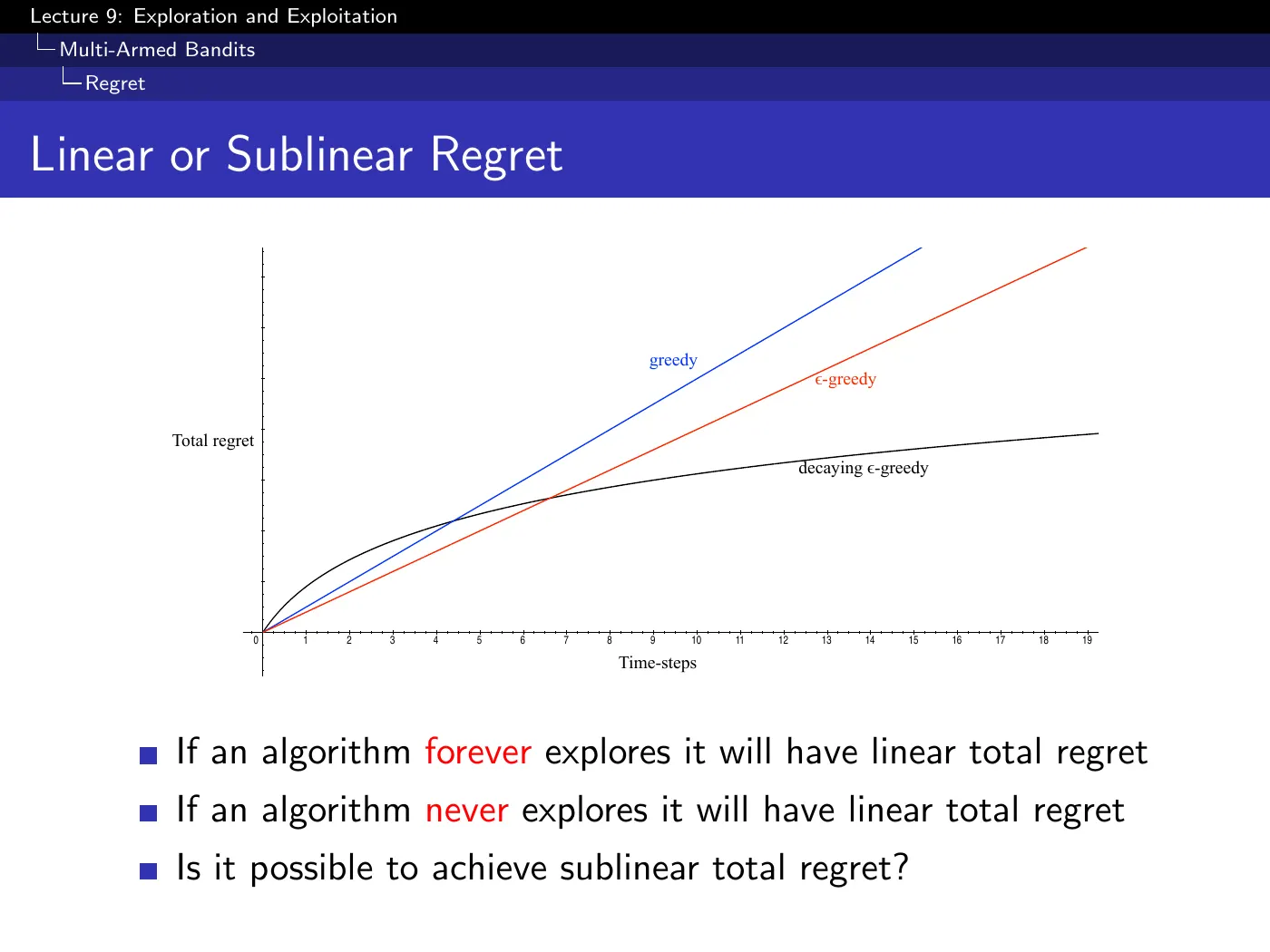
Lecture 9 Exploration and Exploitation, slide 9

Both failure modes are linear, for opposite reasons

Explore forever at a fixed rate and you incur a fixed expected loss every step, forever. The curve has constant slope.
Never explore and you can lock onto a suboptimal arm permanently, incurring that arm's gap every step, forever. Same shape, different cause.
So the target is not "explore less" or "explore more" — it is an algorithm that makes fewer mistakes as it accumulates experience. Read the flattening curve as a falling mistake rate, not as a diminishing amount of exploration.

p.10–11 · Greedy and ε-Greedy ⏱ 23:35

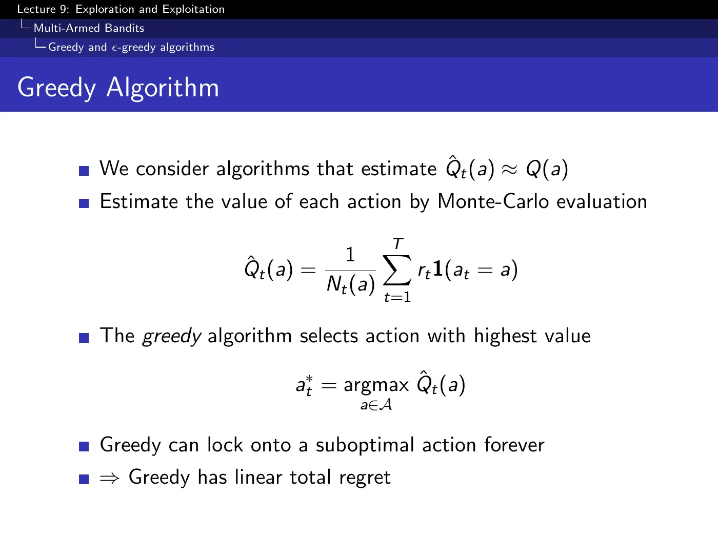
Lecture 9 Exploration and Exploitation, slide 10

Greedy locks on, and the failure is subtler than "it picks the wrong arm". You can try the best arm, be unlucky twice, conclude it is bad, and never revisit it. One bad sample is enough to permanently exclude the optimal action, because nothing in the algorithm ever revisits a rejected belief.

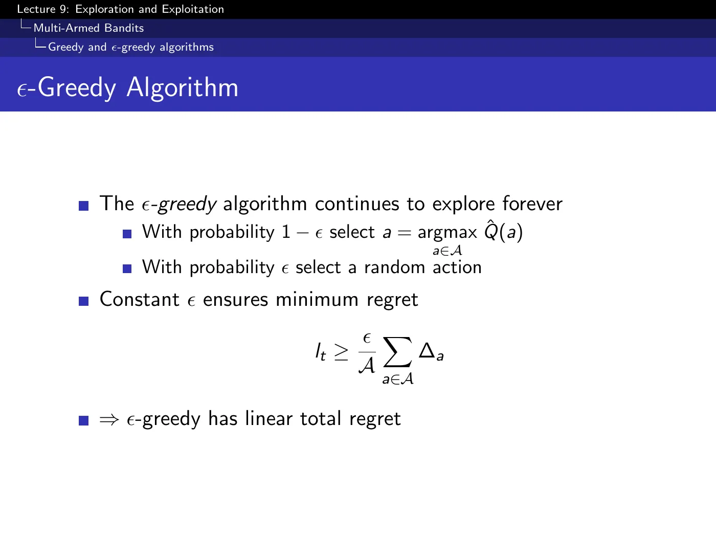
Lecture 9 Exploration and Exploitation, slide 11

$\epsilon$ -greedy fixes that and breaks the other way: with probability $\epsilon$ you draw uniformly, which means you keep deliberately choosing arms you already know are bad. That guarantees a per-step regret floor of at least $\frac{\epsilon}{|\mathcal{A}|}\sum_a\Delta_a$ — hence linear.

p.12 · Optimistic Initialization ⏱ 25:55

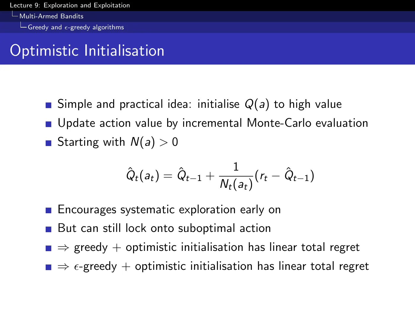
Lecture 9 Exploration and Exploitation, slide 12

Initialize $\hat Q(a)$ to a high value and act greedily. Untried actions look attractive, so early trials push their estimates toward reality. This creates exploration without an ongoing random-action rate, but the initial value and pseudo-count still determine how strong and persistent the optimism is.

The slide's "Starting with

N(a)>0

" is doing hidden work

This is not a detail — it is how you set the strength of your optimism, and the slide never explains it. The clean implementation initializes both the value and the count: initialize as if you had already pulled this arm 100 times and seen the maximum payout every time.
Then the incremental mean $\hat Q_t(a_t)=\hat Q_{t-1}+\frac{1}{N_t(a_t)}(r_t-\hat Q_{t-1})$ moves slowly, and real data has to outweigh that prior before the arm is abandoned. A large $N(a)$ means you have to be very unlucky to lock out the optimal action.
This behaves like a pseudo-count prior: the initial value and count together say how much imaginary evidence must be overcome. For Bernoulli rewards it can be related to prior counts, but it is not automatically the same Bayesian model used later.

Despite the linear-regret verdict, the lecture is emphatic that this is a good idea in practice and hard to beat in many applications. The theoretical failure — you can still be unlucky enough to lock out the best arm — needs bad luck proportional to the confidence you assigned.

p.13 · Decaying ε-Greedy ⏱ 32:02

Lecture 9 Exploration and Exploitation, slide 13

d=\min_{a\mid\Delta_a>0}\Delta_a,\qquad \epsilon_t=\min\left\{1,\frac{c|\mathcal{A}|}{d^2 t}\right\}

The most surprising result in the lecture, and it is about the method everyone dismisses

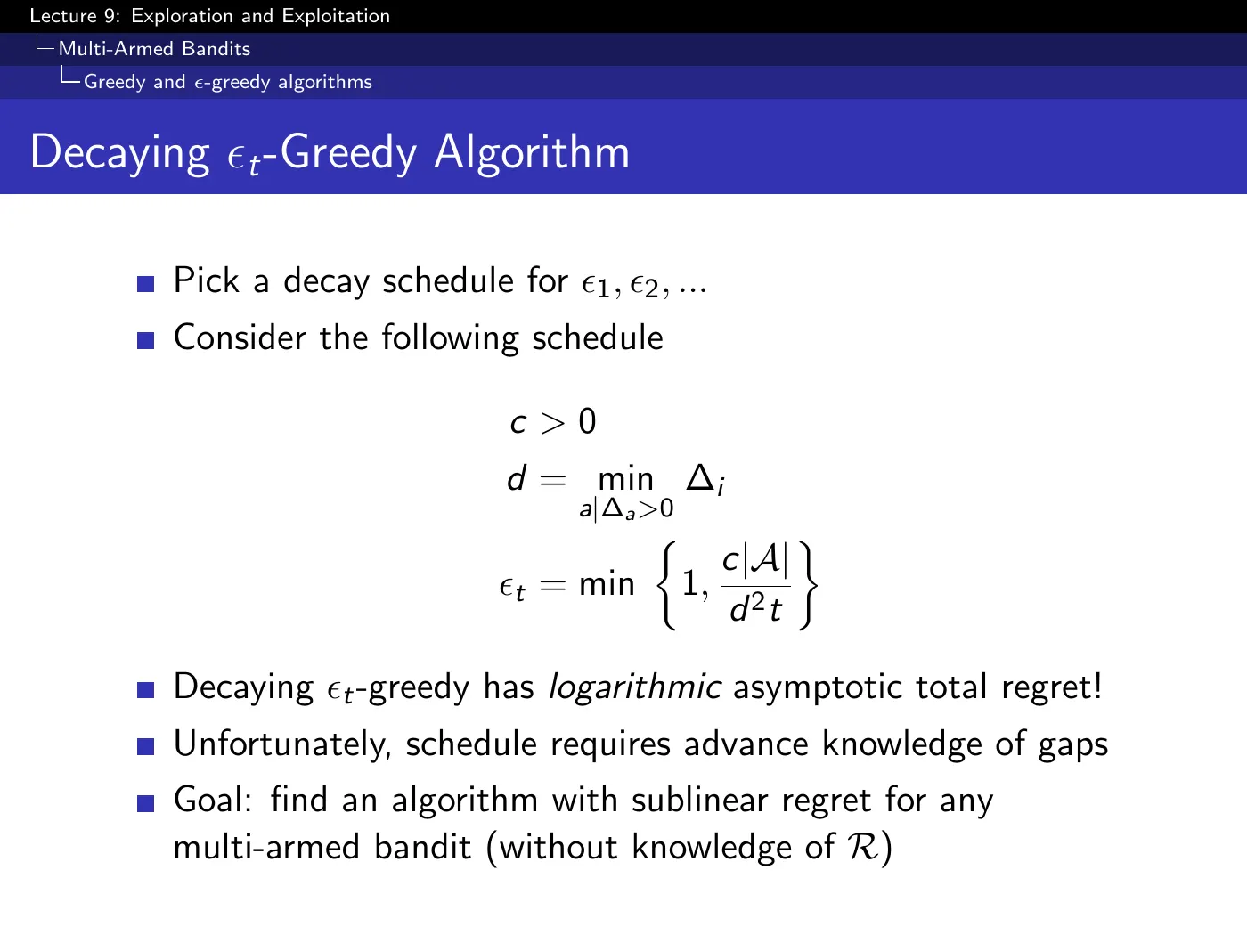
With the right schedule, plain $\epsilon$ -greedy achieves logarithmic asymptotic total regret — which is the best order achievable, up to constants. The naive method was never the problem.
The problem is that the schedule depends on $d$ , the smallest gap — which requires knowing $V^*$ , which is the thing you are trying to learn. The schedule is unimplementable by construction.
So the goal for the rest of the lecture is sharply defined: get this same sublinear regret without advance knowledge of $\mathcal{R}$ . UCB is the answer, and its whole design is "estimate what the ideal schedule would have known."

The specific schedule is less important than its dependence on the unknown smallest positive gap $d$ . That dependence is what makes the theorem explanatory rather than directly implementable.

3 · The lower bound

p.14 · Lai and Robbins ⏱ 36:34

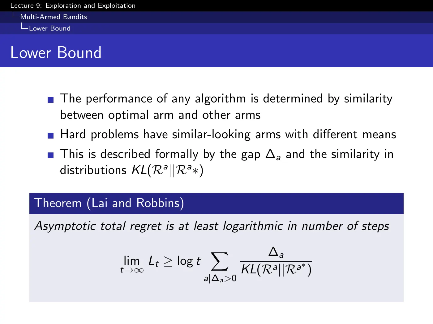
Lecture 9 Exploration and Exploitation, slide 14

\liminf_{t\to\infty}\frac{L_t}{\log t} \;\ge\; \sum_{a:\Delta_a>0} \frac{\Delta_a}{\operatorname{KL}(\mathcal{R}^a\Vert\mathcal{R}^{a^*})}.

The slide compresses the asymptotic notation into $\lim L_t\ge \log t(\cdots)$ , which leaves $t$ on the right side of a limit. The normalized form above is the precise statement. It applies to sufficiently well-behaved, uniformly efficient policies and identifiable reward families; it is not a lower bound on literally every possible algorithm without conditions.

The bound formalizes what makes a bandit hard, and the answer is not what you might guess.

Hardness is similarity, not difference

An easy bandit has one obviously good arm and one obviously bad one — pull each once and you are done.
A hard bandit has arms whose distributions overlap heavily but whose means differ. You cannot tell them apart from a few samples, so you spend a long time misattributing noise.
The two terms capture exactly this. $\Delta_a$ in the numerator: the bigger the gap, the more each mistake costs. $KL(\mathcal{R}^a\Vert\mathcal{R}^{a^*})$ in the denominator: the more similar the distributions, the harder to distinguish, the larger the bound.
A large gap with well-separated distributions is easy despite the gap. A small gap with heavy overlap is where the regret accumulates.

The bound says that logarithmic growth is the best general asymptotic order under those conditions. Matching the order does not settle the constants: an algorithm may still be far from the Lai–Robbins constant.

4 · Optimism in the face of uncertainty

p.15–17 · The Principle and Upper Confidence Bounds ⏱ 39:36

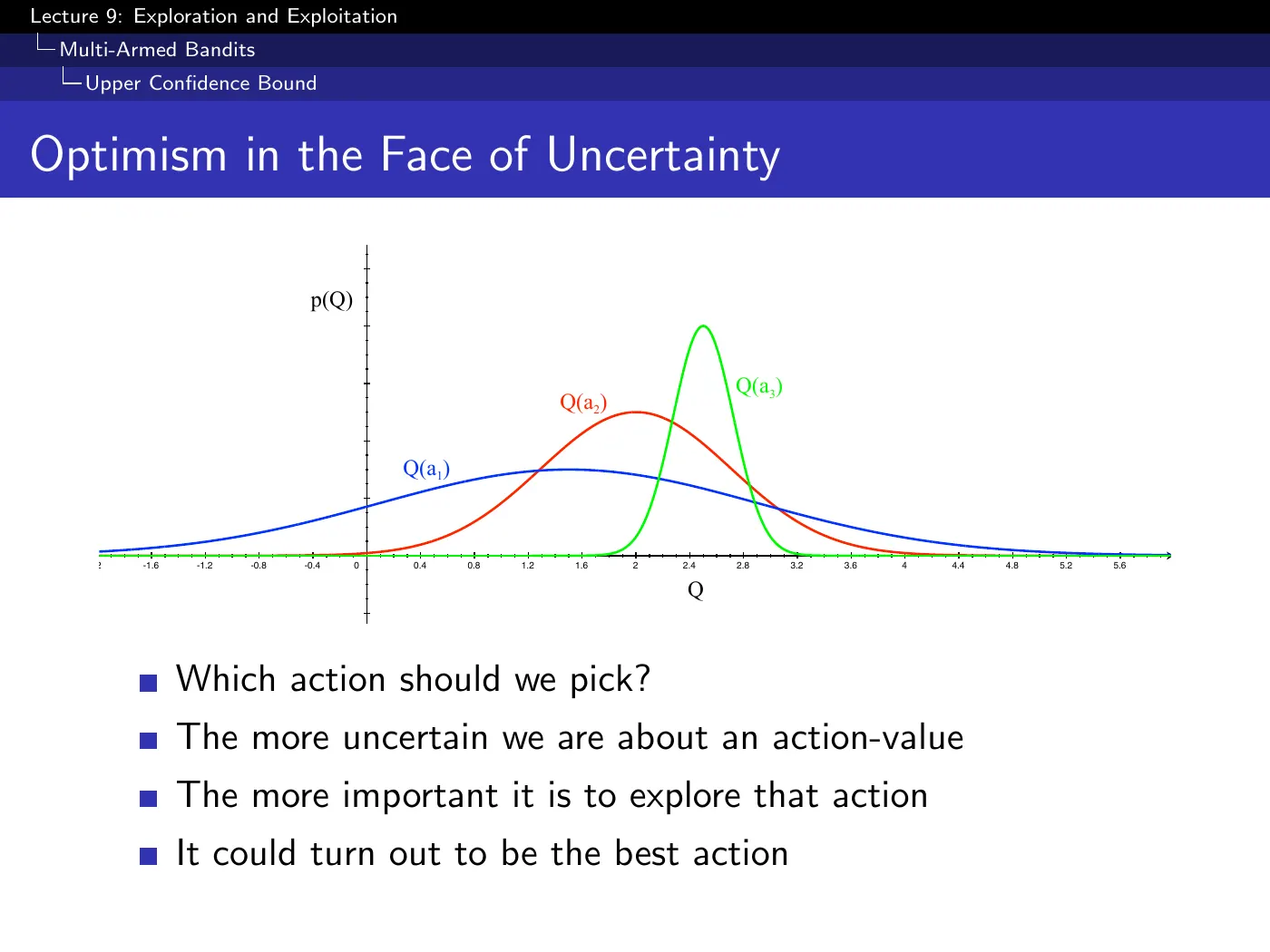
Lecture 9 Exploration and Exploitation, slide 15

Three arms with belief distributions over their values. Green is well-sampled and narrow; blue has been tried twice and is wide. Green has the highest mean.

Pick blue. Not because you think it is better, but because it has the most potential to be better — its tail carries real mass at high values.

Why optimism is not merely optimistic

Sampling an uncertain arm has two possible benefits: if it is good, you discover a better action; if it is bad, repeated evidence shrinks its confidence region. The cost is not literally one-off when rewards are noisy, but a sound confidence rule makes the expected number of suboptimal pulls grow only logarithmically.

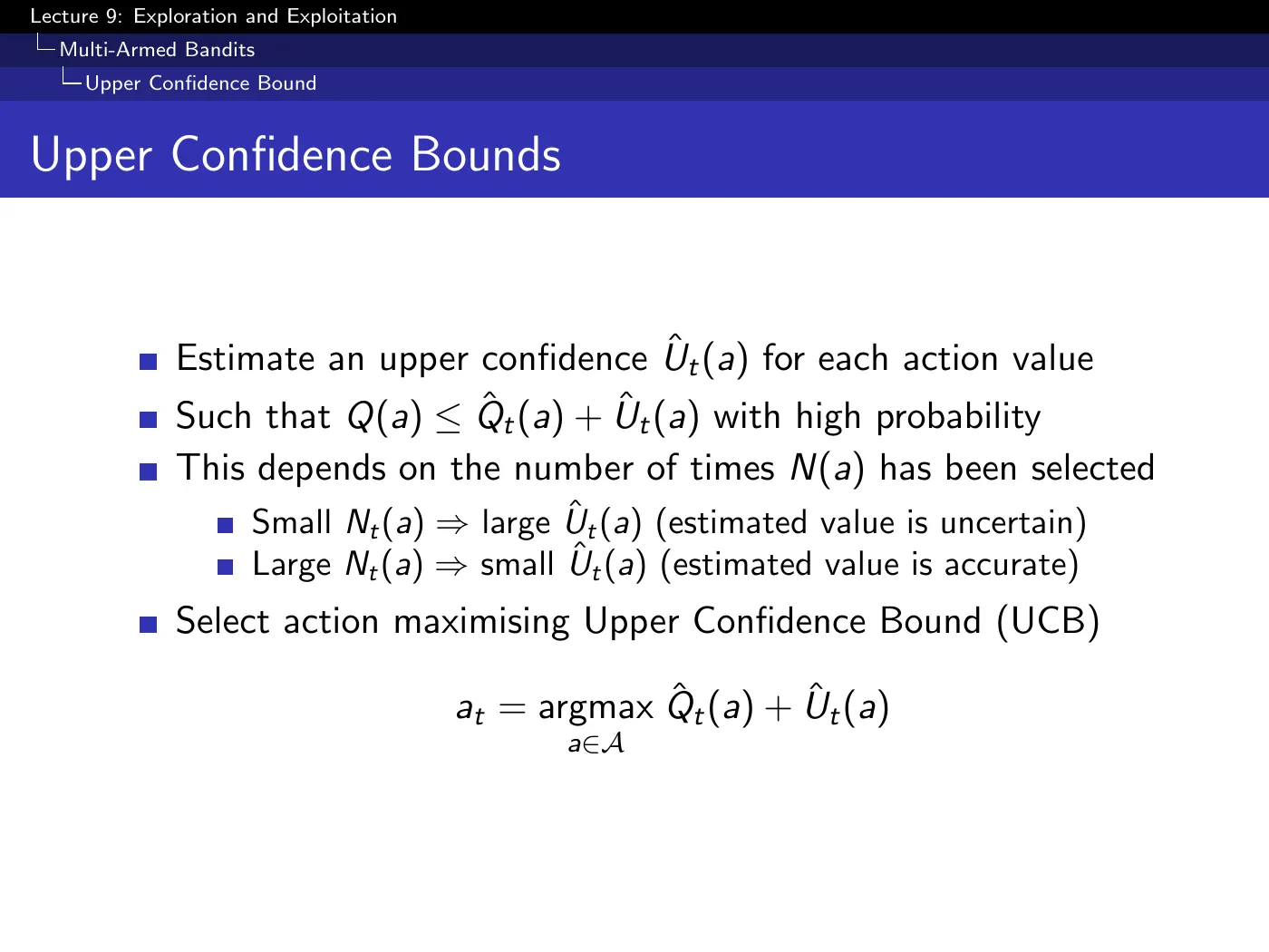
Lecture 9 Exploration and Exploitation, slide 17

a_t=\arg\max_{a\in\mathcal{A}}\;\hat Q_t(a)+\hat U_t(a)

At a fixed global time $t$ , the bonus $\hat U_t(a)$ shrinks as $N_t(a)$ grows. Across time, the $\log t$ term also grows, so a neglected arm's bonus can recover and force another check. UCB therefore makes suboptimal pulls increasingly rare rather than literally turning exploration off once and for all.

p.18–20 · Hoeffding, and UCB1 ⏱ 47:15

Lecture 9 Exploration and Exploitation, slide 18

\mathbb{P}\big[\mathbb{E}[X]>\bar X_t+u\big]\le e^{-2tu^2}

What does Hoeffding's inequality assume? This is the one place to be careful.

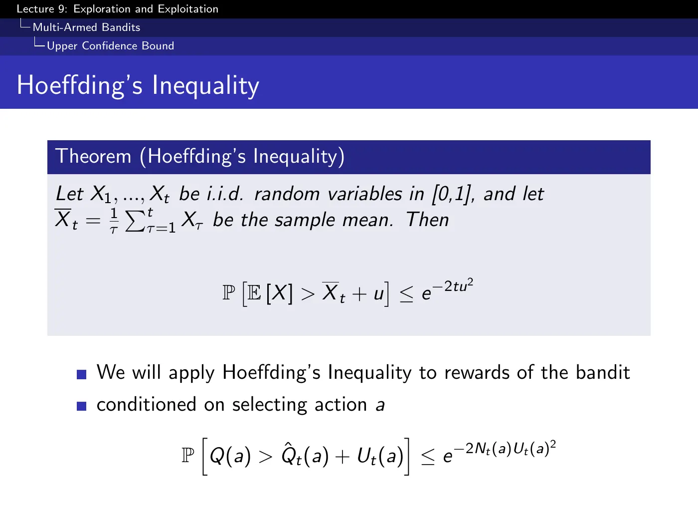
Independent, identically distributed samples from the same arm, with rewards bounded in $[0,1]$ . Conditioned on choosing arm $a$ , its reward law must remain stationary. No symmetry, Gaussianity, or other shape assumption is required.
If your rewards are not in $[0,1]$ , rescale them, which requires knowing $r_{\max}$ and $r_{\min}$ . If the reward is genuinely unbounded, this version does not apply.
That distribution-freedom is exactly why the bound is somewhat weak — assuming nothing means you cannot exploit anything. The Bayesian section buys tightness back by making assumptions.

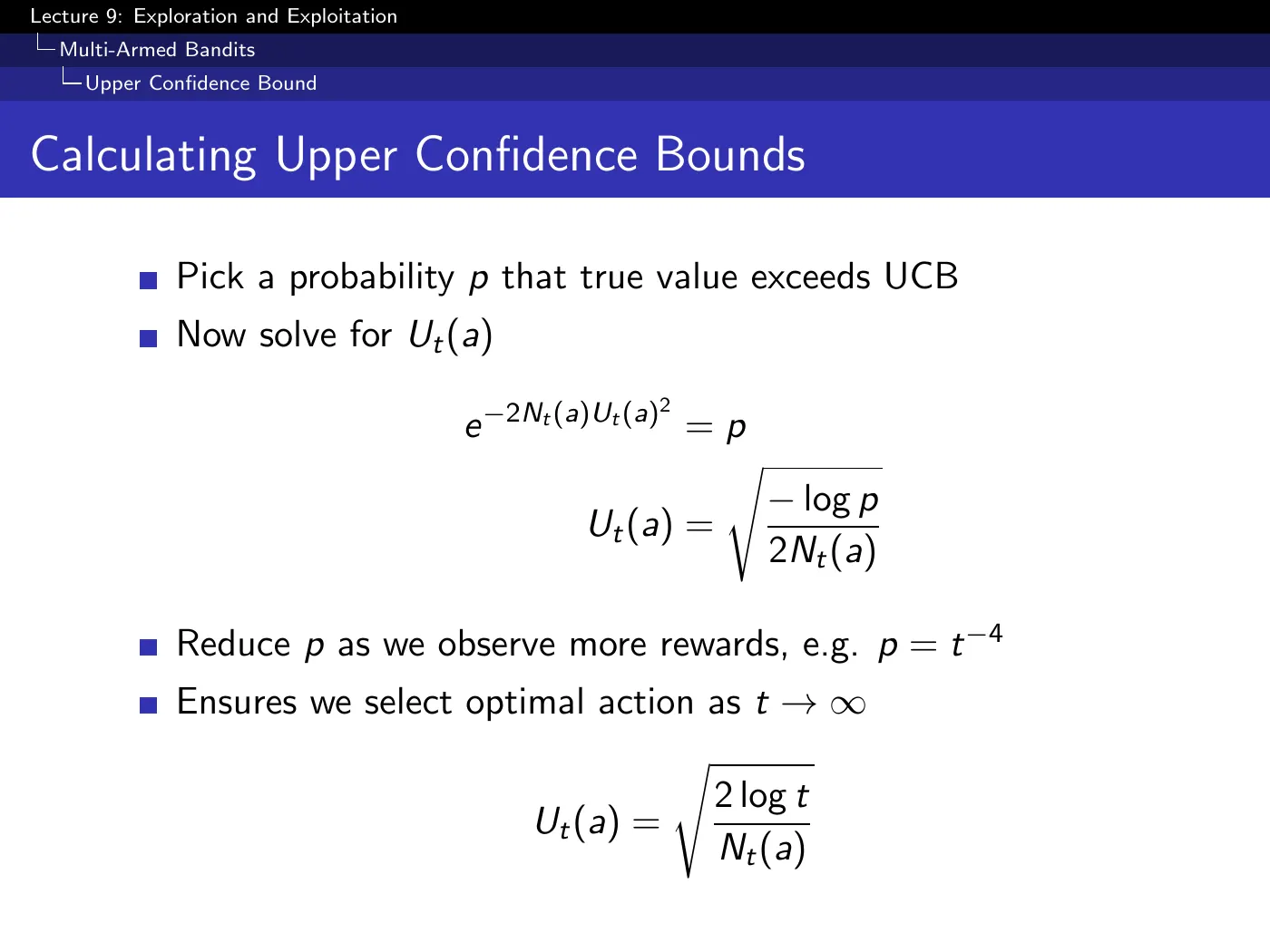
Lecture 9 Exploration and Exploitation, slide 19

The derivation is three mechanical steps — set the right-hand side to $p$ , take logs, solve for $U_t(a)$ :

e^{-2N_t(a)U_t(a)^2}=p\quad\Longrightarrow\quad U_t(a)=\sqrt{\frac{-\log p}{2N_t(a)}}

Then one non-mechanical choice: let $p$ shrink over time, $p=t^{-4}$ , giving $U_t(a)=\sqrt{2\log t/N_t(a)}$ .

That schedule is what converts a one-time confidence statement into a sequential algorithm. If $p$ were fixed, an arm abandoned after an unlucky estimate would keep a fixed bonus and might never become attractive again. Letting $p$ shrink makes the bonus of an under-sampled arm grow slowly with global time, so no arm is permanently discarded merely because of early noise.

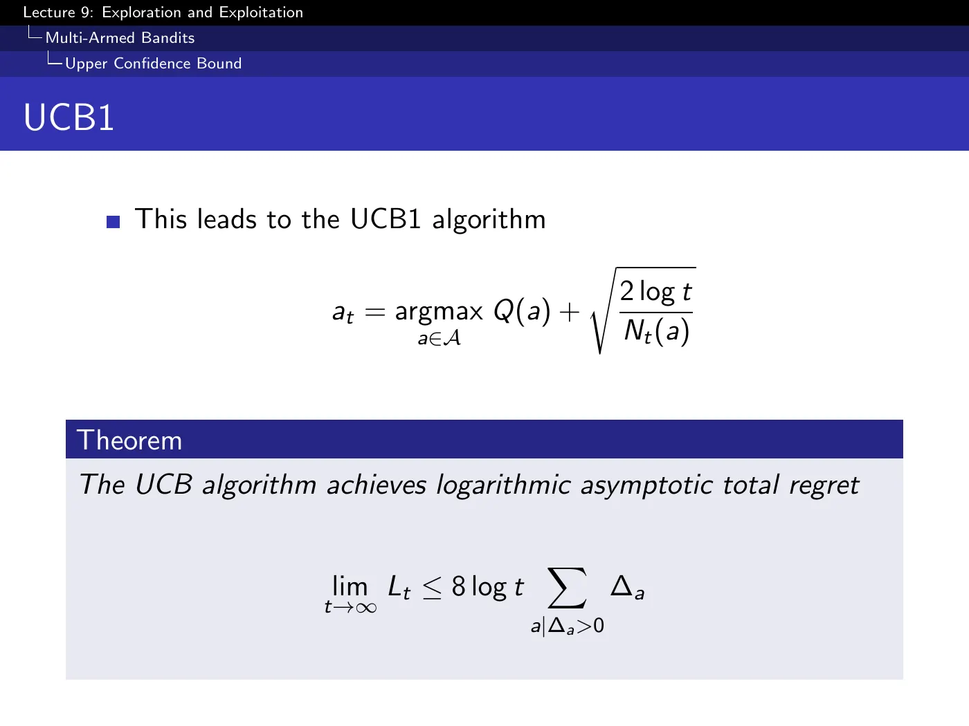
Lecture 9 Exploration and Exploitation, slide 20

a_t=\arg\max_{a\in\mathcal{A}}\;\hat Q_t(a)+\sqrt{\frac{2\log t}{N_t(a)}}.

A standard finite-time reading of the leading regret term is

L_t\;\lesssim\;8\log t\sum_{a:\Delta_a>0}\frac{1}{\Delta_a}+O(1).

The displayed regret formula on p.20 drops the reciprocal

The slide prints $8\log t\sum_a\Delta_a$ . That cannot be the standard UCB1 gap-dependent bound: the number of pulls of a suboptimal arm scales as $O(\log t/\Delta_a^2)$ , so multiplying by its per-pull regret $\Delta_a$ gives $O(\log t/\Delta_a)$ . Read the slide's formula as a typesetting error; the qualitative claim, logarithmic regret, is the part used later.

Read the bonus term structurally: $N_t(a)$ in the denominator means rarely-tried arms get large bonuses; $\log t$ in the numerator means the bonus creeps back up over time for everything, so nothing is ever permanently abandoned.

Compare against Lai and Robbins: UCB1 gets the $\log t$ order but has no $KL$ -adaptive constant — it cannot exploit distributional structure it never assumed. It is optimal in order, not generally asymptotically optimal in constant.

p.21 · UCB vs ε-Greedy in Practice ⏱ 54:50

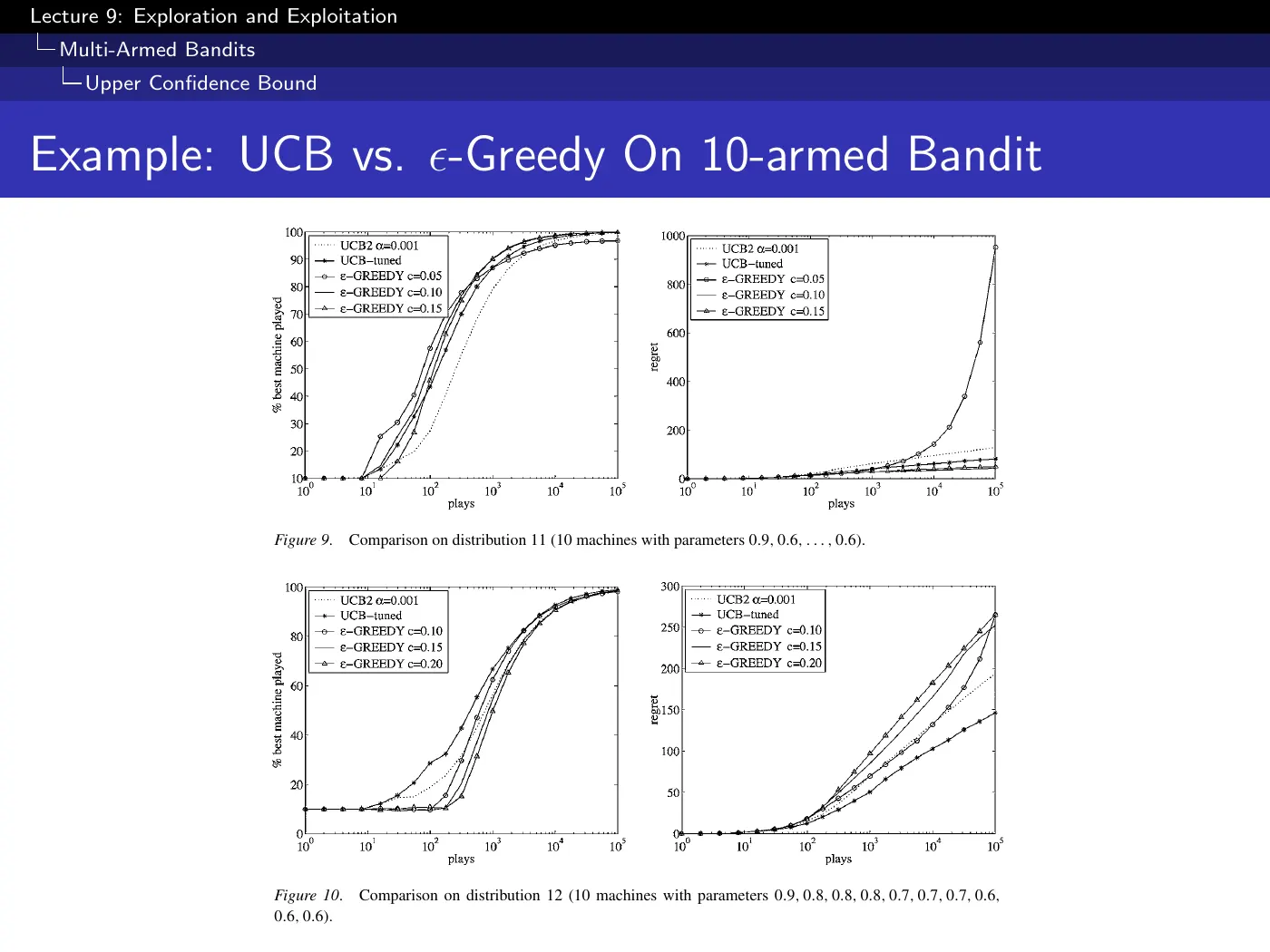
Lecture 9 Exploration and Exploitation, slide 21

Left panels are % best machine played (higher is better); right panels are regret (lower is better).

The correct reading of this figure is not "UCB wins"

A well-tuned $\epsilon$ -greedy does very well — sometimes competitively. The problem is on the right panel, where a badly-chosen $\epsilon$ fails badly.
So the real distinction is not average performance but robustness: $\epsilon$ -greedy has a tuning parameter whose useful value depends on the unknown problem, while the displayed UCB variants need no gap-dependent tuning under their bounded stationary-reward assumptions.
In this experiment the UCB curves approach playing the best arm almost all the time. That is the sublinear-regret behavior made visible; the plot is evidence for these settings, not a universal empirical ranking.

5 · Bayesian bandits and probability matching

p.22–23 · Bayesian UCB ⏱ 57:07

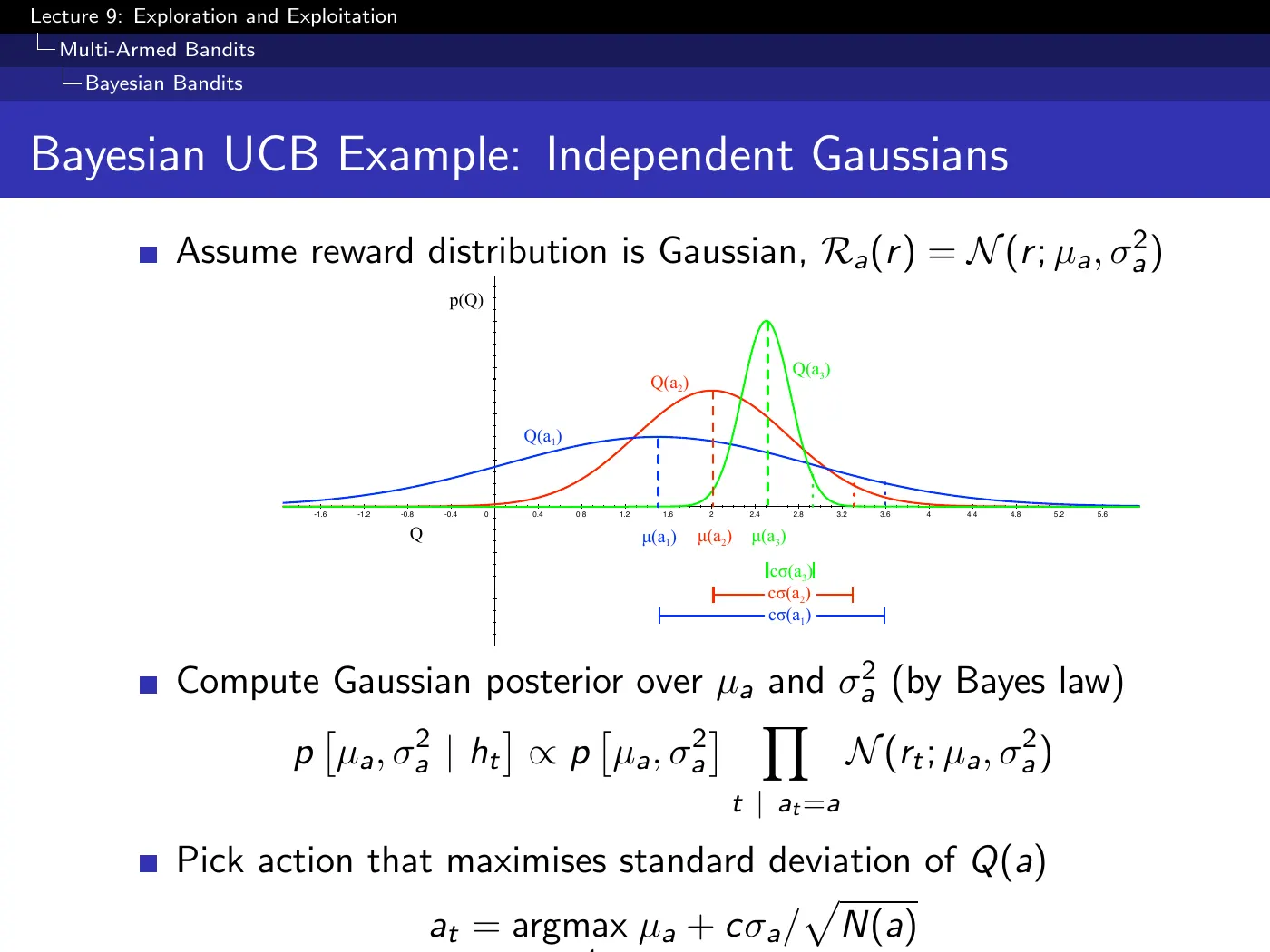
Lecture 9 Exploration and Exploitation, slide 23

a_t=\arg\max_a\;\mu_a+\frac{c\sigma_a}{\sqrt{N(a)}}

Everything so far tracked only means. The Bayesian approach tracks a full posterior — for independent Gaussians, a mean and a variance per arm — and reads the exploration bonus straight off it as some number of standard deviations.

The structural contrast with UCB1 is the point:

	UCB1 (frequentist)	Bayesian UCB
Assumes	rewards bounded	a full prior over $\mathcal{R}$
Tracks	empirical mean and count	a posterior over reward parameters
Bonus from	Hoeffding, a general fact	the posterior's own width
If assumptions are wrong	its stated bound may fail if boundedness fails	the posterior may be confidently miscalibrated

Bayesian bandits are only as good as the prior you put in

With accurate prior knowledge they can beat distribution-free methods because they exploit structure UCB1 refuses to assume. A poor prior or likelihood can instead produce overconfident exploration decisions. UCB1 is more robust to distributional misspecification, though it still relies on bounded or otherwise controlled rewards.
The performance gain and the failure mode come from the same source.

p.24–25 · Probability Matching and Thompson Sampling ⏱ 1:01:45

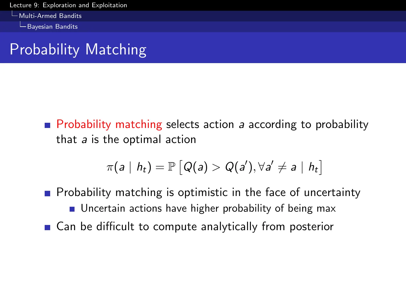
Lecture 9 Exploration and Exploitation, slide 24

Select each action with the probability that it is the best action, $\pi(a\mid h_t)=\mathbb{P}[Q(a)>Q(a'),\forall a'\ne a\mid h_t]$ .

Probability matching gets optimism for free

Nobody wrote an exploration bonus here. An uncertain arm can nevertheless place posterior mass above the current best, so Thompson sampling selects it in proportion to its posterior probability of being optimal. This is not a blanket rule that larger posterior variance always means a larger selection probability; the posterior mean and shape matter too.
Optimistic behavior can therefore emerge from posterior probability matching rather than from an explicit bonus term.

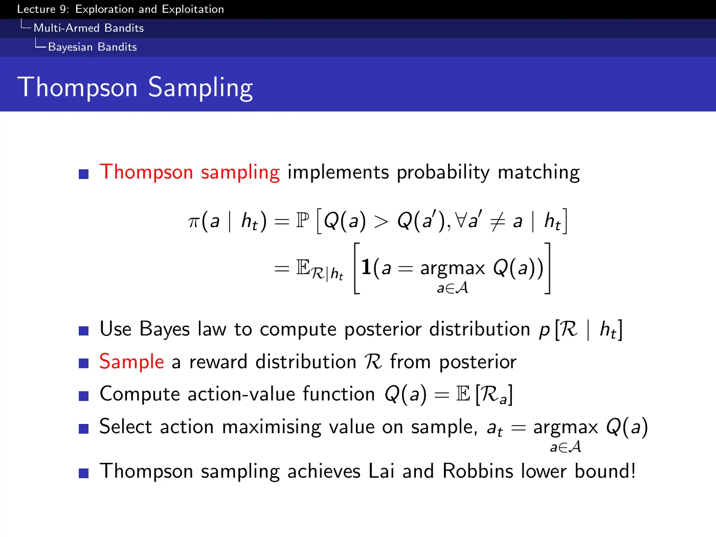
Lecture 9 Exploration and Exploitation, slide 25

The slide gives probability matching in closed form and then observes it is hard to compute. Thompson sampling is the method that makes it trivial: draw one sample from each arm's posterior, and pick the arm whose sample is highest.

Sampling from a distribution and taking the argmax is selecting in proportion to the probability of being the max. No integral, no bonus term, one line of code.

The oldest algorithm here can match the asymptotic lower bound

Thompson sampling dates to the 1930s, predating the formal study of bandits. Under appropriate model and regularity assumptions, asymptotic analyses show it can attain the Lai–Robbins constant; UCB1, as presented here, matches only the logarithmic order.
It has no separate exploration coefficient like Bayesian UCB's $c$ : exploration falls out of posterior sampling. It is not assumption-free or literally parameter-free, because the prior, likelihood, and any model hyperparameters still determine the posterior.

It does not transplant cleanly to full MDPs

Naively sampling a fresh action hypothesis at every step can lose exploration consistency — the same objection raised against $\epsilon$ -greedy at ⏱ 8:22. In an MDP, a standard repair is posterior sampling over an entire MDP or policy for an episode or planning horizon, so the agent tests one coherent hypothesis long enough to reach informative states.

6 · Information state search

p.26–27 · The Value of Information ⏱ 1:08:38

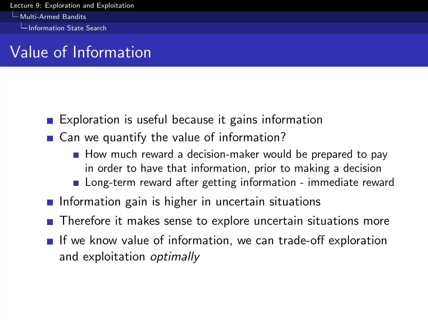
Lecture 9 Exploration and Exploitation, slide 26

Everything before this slide uses a direct action-selection rule. UCB and Thompson sampling can have strong regret guarantees, but they do not explicitly solve the finite-horizon Bayesian question: is one more observation worth its opportunity cost right now?

The reframing: exploration is valuable because it yields information, so price the information in units of reward. How much future reward would you pay, right now, to know what is behind that door? Once you can answer that, the trade-off stops being a heuristic and becomes an optimization.

The price depends on your remaining budget. Information about an arm you can pull only three more times is worth less than the same information with a thousand decisions ahead. Regret algorithms can be analyzed for finite horizons, but the information-state formulation makes the remaining horizon part of the decision problem itself.

Lecture 9 Exploration and Exploitation, slide 27

\tilde{\mathcal{M}}=\langle\tilde{\mathcal{S}},\mathcal{A},\tilde{\mathcal{P}},\mathcal{R},\gamma\rangle

The move: make what you know part of where you are

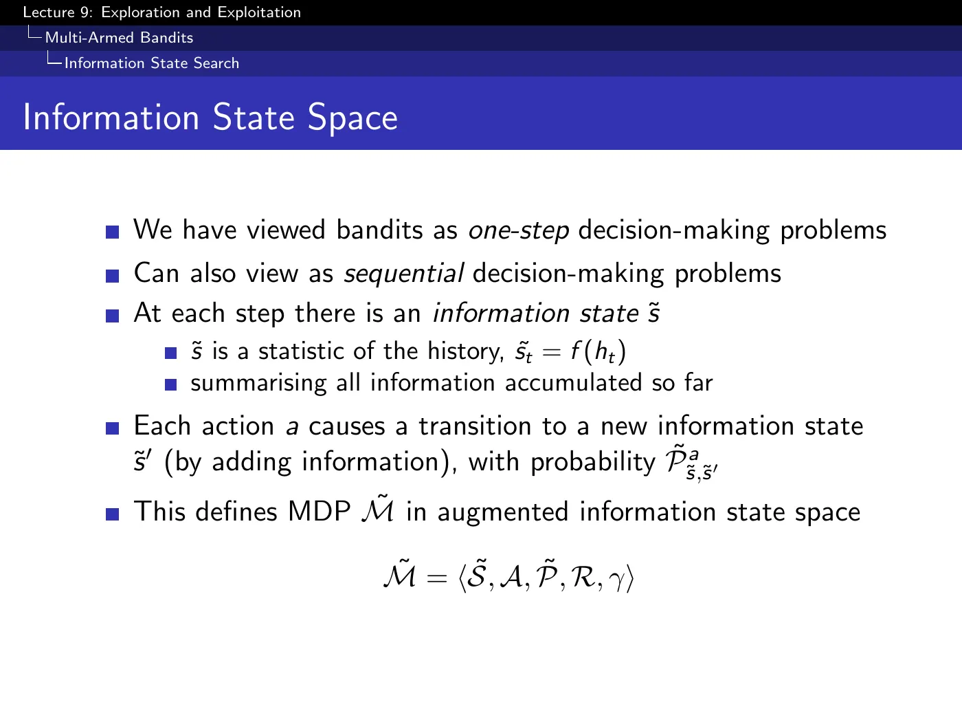
"I have pulled the left lever 3 times and the right lever 5 times" is treated as a state. Pulling a lever leads stochastically to a new information state because the next reward is unknown; the posterior-predictive distribution supplies the transition probabilities.
The consequence is a large simplification: the exploration problem has been converted into a planning problem, and you already know how to solve those. Everything from L3 through L8 now applies — value iteration, Q-learning, MCTS.
There is no exploration-exploitation dilemma inside this MDP. Solve it and the optimal policy is the optimal trade-off. The dilemma was an artifact of not modeling knowledge.

Does the reward function change in the information-state MDP?

No — only the state space is augmented. The rewards are the bandit's original rewards, unchanged.
What changes is the value function, because you are no longer stopping after one step. Value now accounts for the fact that information acquired now yields more reward later. That is where the value of information enters — not through a modified reward signal, but through the horizon.

p.28–32 · Bernoulli Bandits and Gittins ⏱ 1:13:56

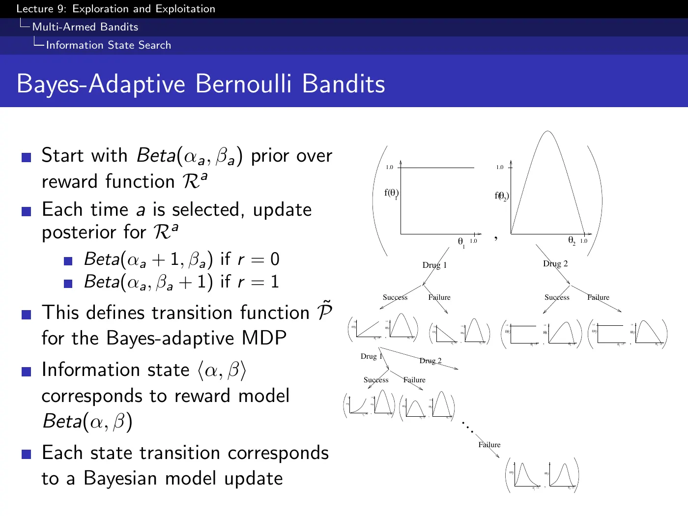
Lecture 9 Exploration and Exploitation, slide 30

For Bernoulli arms the information state is just the two outcome counts $\langle\alpha,\beta\rangle$ , and the posterior is $\operatorname{Beta}(\alpha,\beta)$ . The deck uses the nonstandard local convention $\alpha=$ number of zero rewards and $\beta=$ number of one rewards; many statistics texts use the opposite naming. Follow the deck within this example, but check the convention before reusing a formula elsewhere.

Writing down the counting rule is specifying the transition function

Under the deck's convention, reward $1$ increments $\beta$ and reward $0$ increments $\alpha$ . The update rule identifies the two possible next information states; their probabilities come from the current posterior predictive distribution.
Each transition is a Bayesian model update. Once the prior and likelihood are specified, these information-state dynamics are known even though the arm's true success probability is not.

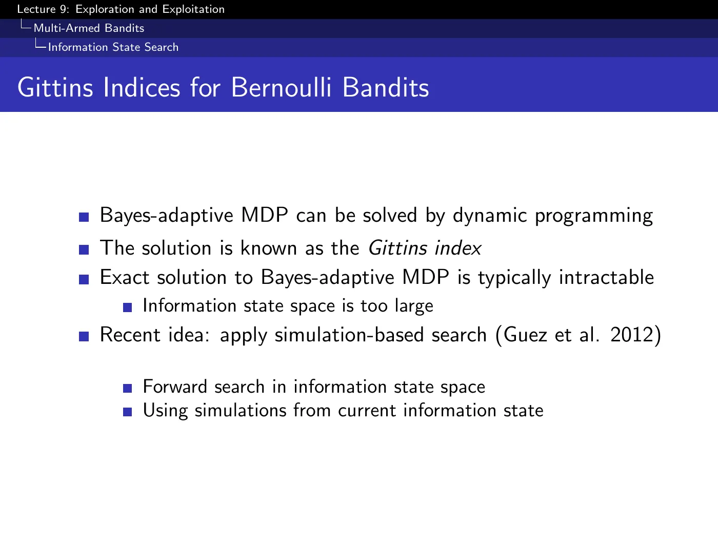
Lecture 9 Exploration and Exploitation, slide 32

For the classical discounted bandit with independent arms, dynamic programming yields the Gittins index — a Bayes-optimal policy under its prior and problem assumptions. It is not a universal index theorem for arbitrary contextual, finite-horizon, or coupled bandits.

And intractable, because the information state space is enormous. The escape route is the previous lecture: simulation-based search (Guez et al. 2012), forward search from the current information state → Lecture 8 · Integrating Learning and Planning. You blow up the state space and then refuse to enumerate it, exactly as MCTS refuses to enumerate a game tree.

7 · Contextual bandits

p.33 and p.38 · The Problem, and Front-Page News ⏱ 1:28:28

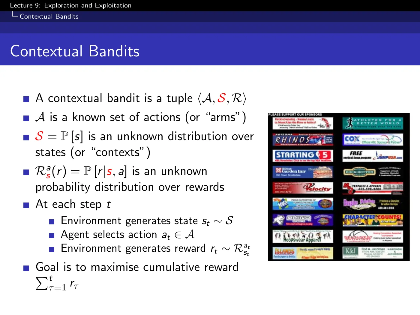
Lecture 9 Exploration and Exploitation, slide 33

Add a state — a context — that you observe before choosing, and that shapes which action is best. $\langle\mathcal{A},\mathcal{S},\mathcal{R}\rangle$ : still one step, still no transitions, but now the reward depends on who showed up.

This is the halfway house between bandits and MDPs, and the lecture flags it as one of the most commercially successful applications of machine learning — banner ad and news placement, where the context is what you know about the arriving user.

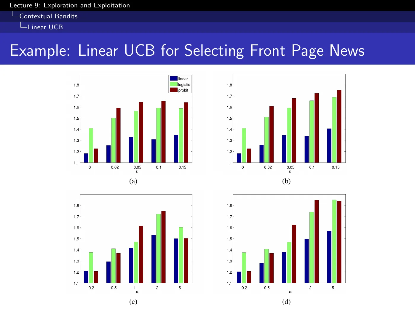
Lecture 9 Exploration and Exploitation, slide 38

The Yahoo front-page news result: choose which article to show based on user statistics, using a UCB-style method.

The solution slides here are deliberately skipped in the lecture

p.34–37 develop LinUCB — linear regression for $Q_\theta(s,a)=\phi(s,a)^\top\theta$ , then a confidence ellipsoid around $\theta$ giving the bonus $c\sqrt{\phi(s,a)^\top A^{-1}\phi(s,a)}$ — and the lecture explicitly leaves them as reading, marking them non-examinable.
They are covered in Gaps to close on your own below with the parts worth knowing.

8 · Back to MDPs

The video discusses p.42 before p.39–41. The order below follows the PDF, so the timestamps intentionally move from ⏱ 1:34:37 back to ⏱ 1:32:19 once.

p.39–41 · Optimistic Initialization in MDPs ⏱ 1:34:37

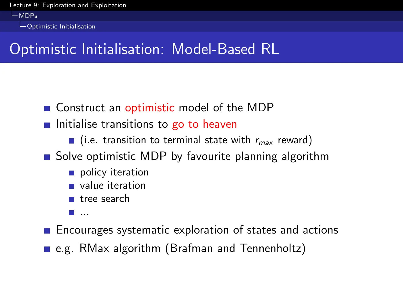
Lecture 9 Exploration and Exploitation, slide 41

Model-free: initialize $Q(s,a)$ to $r_{\max}/(1-\gamma)$ and run anything. Model-based is the interesting one, and the mechanism deserves spelling out because the slide compresses it to one line.

"Transition to heaven" — optimism that generates a plan, not just a preference

Point every unknown transition at a fictitious terminal state paying $r_{\max}$ . Then run any planner from L3.
What happens is better than exploration: the planner computes a route to the unknown state, because it believes the maximum reward is there. You arrive, discover it is ordinary, update the model, re-plan — and the planner routes you to the next unexplored state.
The difference from $\epsilon$ -greedy is total. $\epsilon$ -greedy hopes to stumble into unvisited states by random perturbation; this deliberately navigates to them, across many steps if necessary, and then systematically removes each fictitious reward as it is disproved. This is the RMax algorithm.

p.42 · Upper Confidence Bounds in MDPs ⏱ 1:32:19

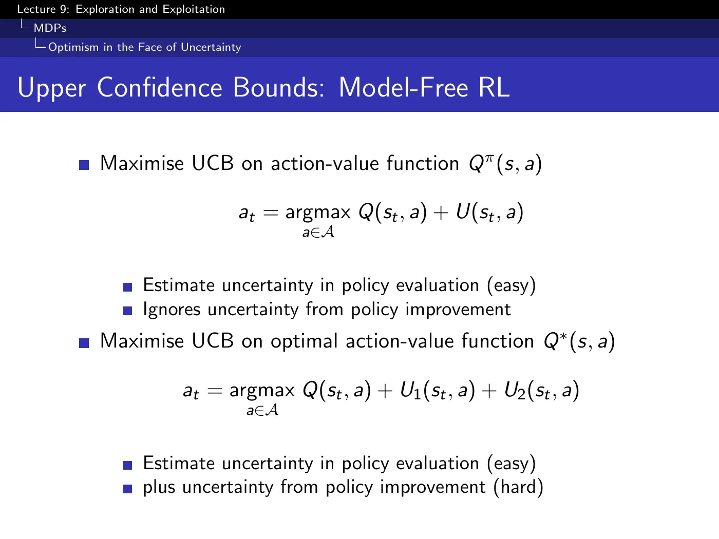
Lecture 9 Exploration and Exploitation, slide 42

The slide marks one term "easy" and the other "hard" without explaining why, and the distinction is the most important thing on it.

In an MDP your

Q

estimate can be wrong in two independent ways

$U_1$ — policy evaluation uncertainty. You have not sampled enough to know $Q^\pi$ for your current policy. This is the bandit problem, and Hoeffding-style bounds handle it. Easy.
$U_2$ — policy improvement uncertainty. Your current policy is not final; it will improve, and $Q^*$ is higher than $Q^\pi$ by an amount you do not know. Estimating how much better you are going to get requires reasoning about your own future learning. Hard.

Bandits have only $U_1$ , because there is no policy to improve — this is precisely what the one-step setting removes. Every MDP exploration method that transplants a bandit bound is quietly ignoring $U_2$ , and that is why theoretical guarantees are so much weaker here.

p.45–46 · Information State Search in MDPs ⏱ 1:36:10

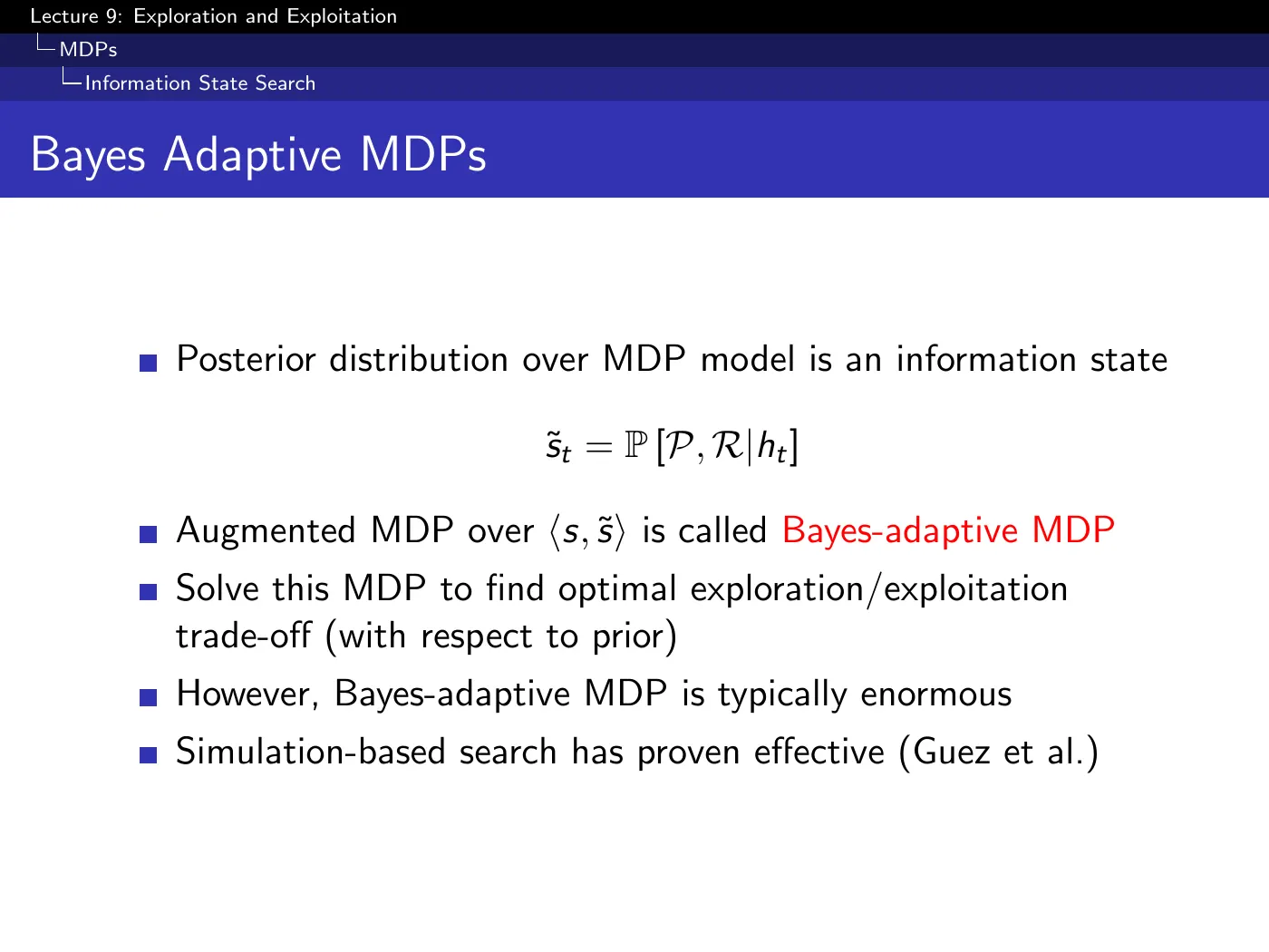
Lecture 9 Exploration and Exploitation, slide 46

\tilde s_t=\mathbb{P}[\mathcal{P},\mathcal{R}\mid h_t]

Augment the state to $\langle s,\tilde s\rangle$ — where you are, plus what you know. The posterior over models is the information state, and the result is the Bayes-adaptive MDP, whose optimal policy is the optimal exploration-exploitation trade-off with respect to your prior.

The same two facts as the bandit case, one lecture later and much worse: it is exactly right, and it is enormous. Simulation-based search is again the practical route, and the caveat is stated outright — it has worked on problems of moderate complexity and has not been scaled to genuinely challenging MDPs.

p.47 · Conclusion ⏱ 1:37:40

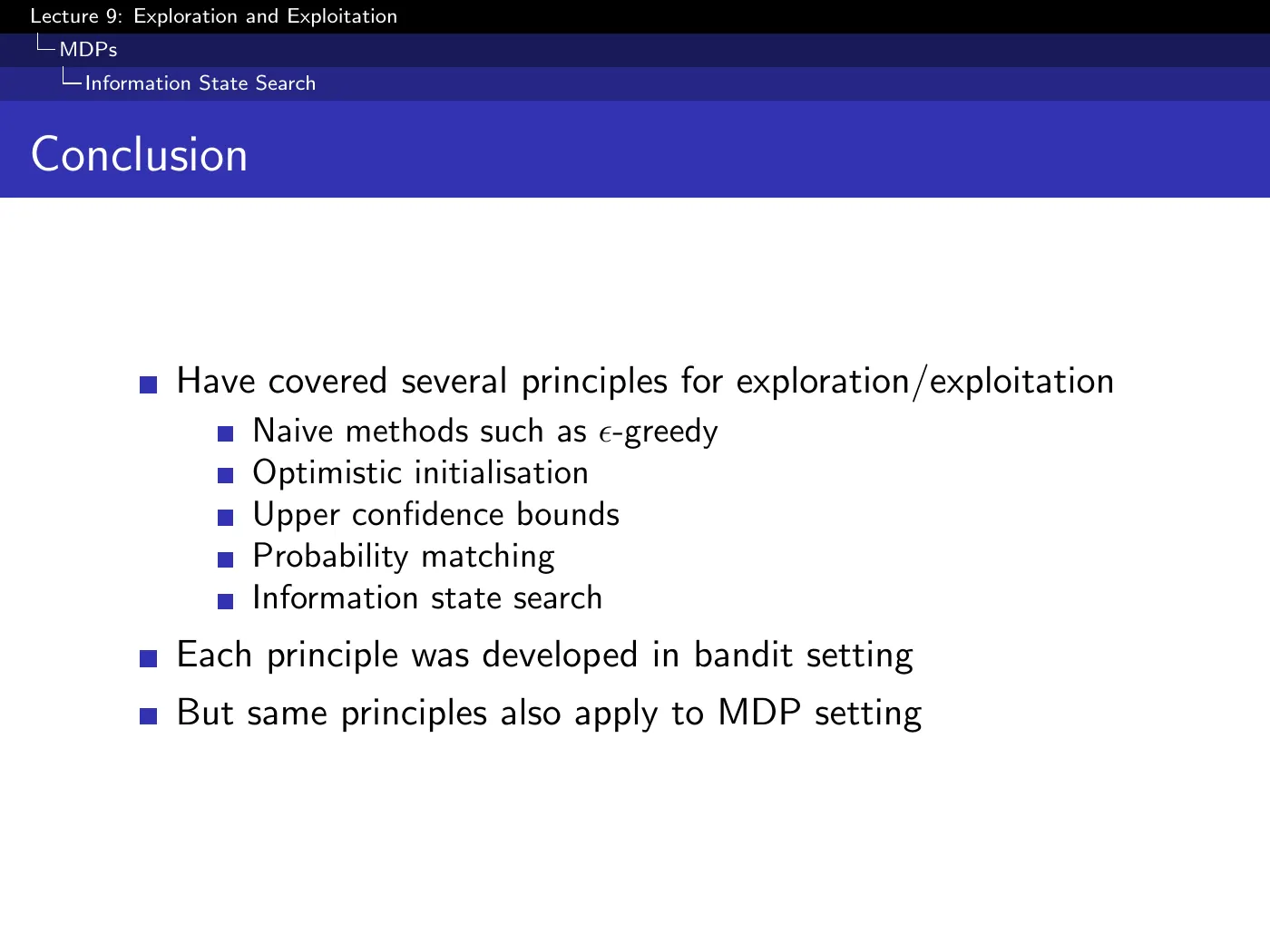
Lecture 9 Exploration and Exploitation, slide 47

Two axes: five principles, three settings. Each principle was developed in the bandit column and transplanted rightward — which is the retroactive justification for spending an hour on a one-step problem.

What this lecture does not give you, and it matters for real robots

The lecture pauses to ask what is wrong with optimism, and the two answers are worth more than most of the theory:

Large or continuous action spaces. A separate confidence bonus for every action no longer scales, and “try each uncertain action” is impossible. Useful optimism then needs structural assumptions that generalize uncertainty across actions.
No safe exploration. Optimism deliberately drives you toward the least-known states — which is exactly where the catastrophes are. Practitioners often do the opposite, staying near regions known to be safe. You do not want to crash your helicopter.

Systematic exploration of the state space is the right objective when mistakes are cheap. When they are not, every principle in this lecture points the wrong way.

Study checklist

Close the note and answer these in your own words. Reopen only the section linked after the question.

Write the regret decomposition and explain what “counts × gaps” reveals. → 1 · The dilemma and the yardstick
Why do greedy and fixed- $\epsilon$ policies both have linear regret for opposite reasons? → 2 · Why the naive methods fail
Why is the logarithmic decaying- $\epsilon$ result not directly implementable? → p.13 · Decaying ε-Greedy ⏱ 32:02
State the normalized Lai–Robbins lower bound and its main conditions. → 3 · The lower bound
Derive the UCB1 bonus from Hoeffding's inequality and explain the roles of $N_t(a)$ and $\log t$ . → p.18–20 · Hoeffding, and UCB1 ⏱ 47:15
What typesetting error appears in the p.20 regret formula? → p.18–20 · Hoeffding, and UCB1 ⏱ 47:15
How do Bayesian UCB and Thompson sampling use a posterior differently? → 5 · Bayesian bandits and probability matching
Why is an information-state transition stochastic even though the Bayesian update rule is known? → 6 · Information state search
Under what problem assumptions is the Gittins index Bayes-optimal? → p.28–32 · Bernoulli Bandits and Gittins ⏱ 1:13:56
How does LinUCB generalize uncertainty across contexts and actions? → Gaps to close on your own
Why can an optimistic model plan a path to an unknown state while $\epsilon$ -greedy cannot? → p.39–41 · Optimistic Initialization in MDPs ⏱ 1:34:37
Why do continuous actions and safety constraints require exploration ideas beyond this lecture? → p.47 · Conclusion ⏱ 1:37:40

Gaps to close on your own

Slides p.34–37 are skipped — LinUCB for contextual bandits

The lecture presents the contextual bandit problem and the Yahoo result, then explicitly defers the solution methods to reading and marks them non-examinable.

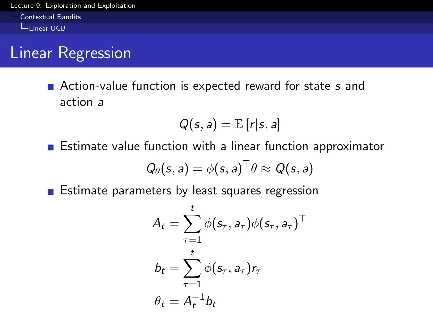
Lecture 9 Exploration and Exploitation, slide 34

The chain is short and worth following. Estimate $Q_\theta(s,a)=\phi(s,a)^\top\theta$ by least squares, $\theta_t=A_t^{-1}b_t$ with $A_t=\sum_\tau\phi\phi^\top$ — the same $O(N^3)$ machinery as LSTD in L6.

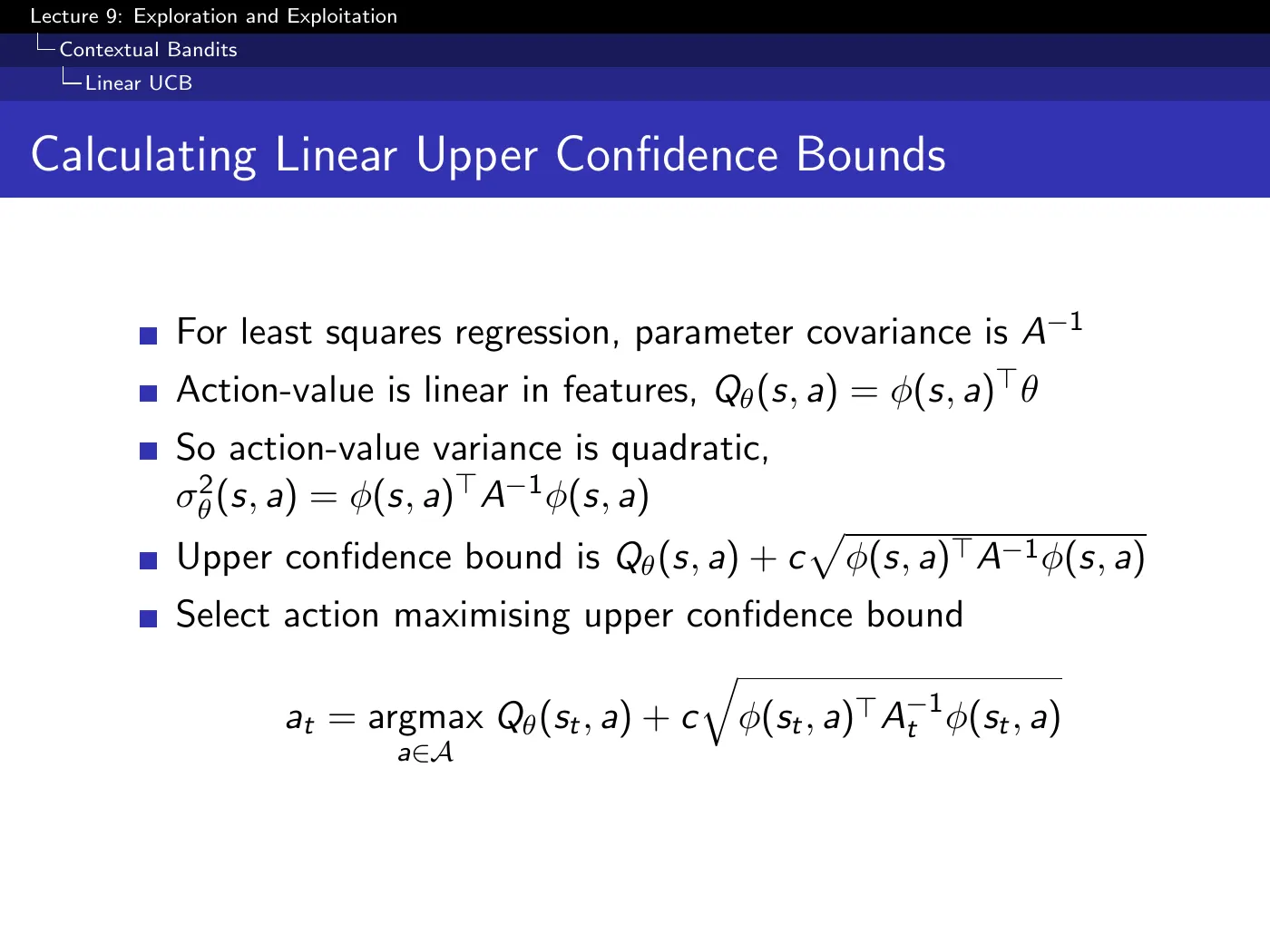
Lecture 9 Exploration and Exploitation, slide 37

Under the regularized linear model and controlled-noise assumptions used by LinUCB, $A^{-1}$ determines the shape of a confidence ellipsoid. The resulting action uncertainty has the quadratic form $\phi(s,a)^\top A^{-1}\phi(s,a)$ , up to the confidence-scale constants, and the bonus is proportional to its square root. This uncertainty is not “free” for arbitrary least squares; it depends on the statistical assumptions behind the confidence set.
This is the natural generalization of UCB to function approximation, and the reason it deserves the reading time is that it is what actually runs in production ad and content-recommendation systems.

UCT is not in this lecture — it is defined in L10. The L8 note originally flagged UCT as material L9 would supply; it does not. This deck develops UCB1 for bandits and mentions MCTS only as the tractable approximation to information-state search. L10 p.37 gives it: UCT is MCTS with every tree node treated as its own bandit, using UCB1 (p.20 here) to select among children — and self-play UCT converges on the minimax values in perfect-information zero-sum two-player games. For the guarantees, Kocsis & Szepesvári (2006).
Slides p.43–44 have no corresponding discussion. Bayesian model-based RL and Thompson sampling for MDPs are stated on slides but passed over in the video — the lecture goes from RMax straight to information state search. They are the direct MDP analogues of p.22–25: maintain a posterior over $\langle\mathcal{P},\mathcal{R}\rangle$ , sample a whole MDP from it, solve that MDP, act optimally for the sample.
The UCB1 regret bound is not derived. The constant $8$ is asserted. If you want it, the source is Auer, Cesa-Bianchi & Fischer (2002).
Gittins indices are named, not computed. You are told the DP solution exists and is called this; no construction is given.
Safe exploration. Raised as a serious practical objection and then left open — the lecture offers no method, only the observation that industry often inverts the principle.
Finite budgets. Acknowledged as something UCB and Thompson sampling get wrong, and as something information-state search handles correctly, but no worked treatment.
Softmax exploration is mentioned repeatedly as a random-exploration alternative to $\epsilon$ -greedy and never analyzed; the lecture asserts it is also linear-regret without showing it.

Language notes

Phrasings worth stealing for your own technical writing and talks:

Expression	Use
the best long-term strategy may involve short-term sacrifices	naming a trade-off without moralizing about it
opportunity loss	the cost of not having chosen the best available option
lock onto a suboptimal action	a process that commits early and never revisits
optimism in the face of uncertainty	prefer what you know least about
until proven otherwise	an assumption held only until evidence displaces it
give or take a constant factor	conceding looseness while keeping the claim
it comes out in the wash	a parameter that calibrates itself, needing no tuning
this is a heuristic	flagging that a method behaves well without being justified
only as good as the knowledge you put into them	a method whose performance is bounded by its assumptions
you don't want to crash your helicopter	grounding a theoretical objection in a concrete cost