Notes·Paper
Lee 2020 · Prerequisites — Lecture Notes
Paper: Lee 2020 - Learning Quadrupedal Locomotion over Challenging Terrain · Before this: Hwangbo 2019 - Learning Agile Motor Skills (ANYmal) · Needed for the TRPO chapter (notes ready, not yet studied): Lecture 7 · Policy Gradient (policy gradient; §2 here only adds TRPO on top of it) · Korean reference copy: Lee 2020 - Prerequisites Lecture Notes (Korean)
How to read. This is not a summary of the paper. It teaches the five things the paper assumes and never explains, in the order the paper needs them, and it stops where the paper starts explaining itself. Read one chapter, then the pages named in its headings with the paper open. Every chapter walks the same path: problem → definition → obstacle → mechanism → correctness → conditions. Page numbers follow the arXiv preprint PDF; "S3" means supplementary section S3.
If Silver L7 is not done yet. Only §2 depends on it.
- Read everything except §2: The one idea, §1, §3, §4, §5, §6, and the appendices (A, B).
- Silver L7 §5–§8: score function, policy gradient theorem, actor-critic, advantage and baseline. The deterministic policy gradient in §9 is not needed here.
- §2, which then reads as one page added on top of L7.
- The paper.
Reading §2 before L7 gives the picture but not the derivation: it will tell you that the step is measured in KL and taken along the natural gradient, but the advantage , the score function, and the claim that the surrogate's gradient at is the policy gradient all come from L7.
Priority marks follow Learning Philosophy: 🔴 practice-critical · 🟡 JIT standby · ⚪ concept anchor.
Highlights: definition or core claim · intuition, mechanism, how to read · the paper's own words · caveat or condition.
The one idea
Hwangbo 2019 trained one network by reinforcement learning on the observation the robot can actually measure, and it worked on flat ground.
On rough terrain the same recipe stalls. The paper reports the failure in one sentence (p. 3): trained directly by RL, the proprioceptive network did not learn to walk within a reasonable time budget because "the supervisory signal was sparse." The reading developed in §3 is that with proprioception alone the network has to solve two problems at once, what is the ground doing and what should the legs do, and a scalar reward per step is too little signal to learn both.
Lee 2020 separates the two problems.
- A teacher is trained by RL in simulation with the ground truth handed to it as input (terrain shape under each foot, contact states and forces, friction, external pushes). It only has to learn what to do.
- A student is trained by supervised imitation to reproduce the teacher's actions and the teacher's internal summary of the ground truth, from a two-second window of proprioceptive history. It only has to learn to infer what the ground is doing.
- A terrain curriculum chooses the terrains both are trained on. A particle filter tracks the set of terrains that are currently hard but passable, and follows that set as the policy improves.
Under all three sits the same motion machinery as before, plus one addition: the network does not output joint targets but modulates a fixed periodic foot trajectory, which is turned into joint targets by inverse kinematics and tracked by joint PD control through the actuator net.
| Paper piece | Where | Prerequisite it assumes | Chapter |
|---|---|---|---|
| Motion generation and tracking (Fig. 4C) | p. 8, S3 | trajectory generators as motion priors, phase variables, yaw-only frames, analytic inverse kinematics | §1 |
| Teacher training | p. 8, S4, Table S7 | Gaussian policies, policy gradient, TRPO's KL trust region | §2 |
| Teacher → student (Fig. 4A) | pp. 6, 8–9, S9 | privileged information, behavior cloning, covariate shift, DAgger | §3 |
| Student architecture | pp. 3, 9, Tables S5–S6, S8 | partial observability, causal and dilated 1-D convolution, TCN | §4 |
| Terrain curriculum (Fig. 4B) | p. 9, S2, S5–S6, Algorithm S1 | Bayes filters, importance weights, SIR particle filter | §5 |
| Ablations and analysis | pp. 10–12, S7 | seeds and confidence intervals, decoder probes, Gaussian NLL, saliency | §6 |
Everything unusual in this paper follows from one decision: training is split into a stage that is allowed to cheat and a stage that is not. Because the teacher will never run on hardware, its observation may contain anything the physics engine knows; its action can be evaluated at any state the student wanders into, which is what DAgger needs (§3); and the terrains it trains on can be scored by ground-truth success, which is what the curriculum needs (§5). The rule of Sensors vs Simulator in Robot RL still binds the student. It is the teacher that is exempt.
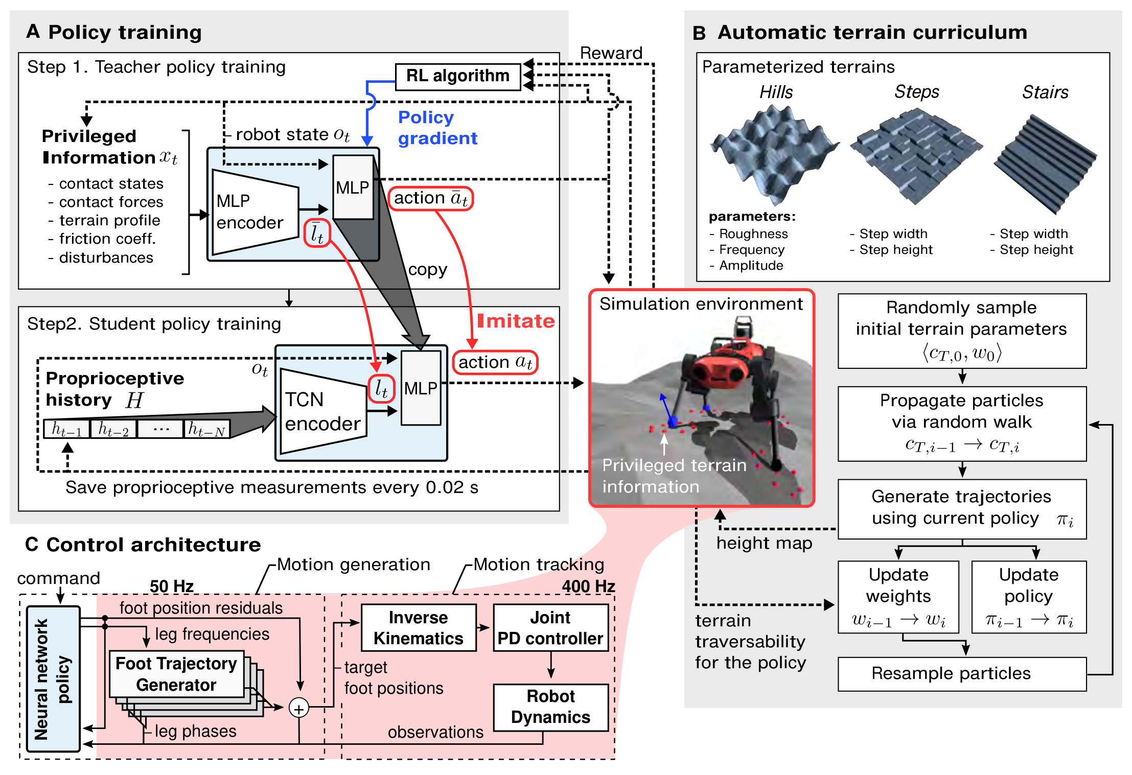
Fig. 4 (p. 7). Read it A → C → B. A: the teacher (top) takes the robot state and the privileged information , compresses into a latent , and outputs an action ; the student (bottom) takes and a proprioceptive history and is trained to output the same and . The starred head layers are copied from teacher to student. C: what an action is: leg frequencies and foot position residuals feeding four foot trajectory generators, then inverse kinematics and joint PD control. B: the terrains are parameterised, and a particle filter over their parameters decides which ones to train on.
Contents
- 1 · Motion prior: phase, trajectory generator, horizontal frame, inverse kinematics
- 2 · Teacher: from policy gradient to TRPO
- 3 · Privileged learning: teacher, student, and DAgger
- 4 · Memory: partial observability and the TCN
- 5 · Curriculum: from Bayes filter to particle filter
- 6 · Reading the evidence
- Appendix A · Deep-learning vocabulary in Tables S5–S9
- Appendix B · Notation cheat sheet (S1)
- Study checklist
- Gaps to close on your own
- Language notes
1 · Motion prior: phase, trajectory generator, horizontal frame, inverse kinematics
🔴 for the trajectory-generator idea and the phase variable · 🟡 for analytic inverse kinematics
p.8 · Why the network does not output joint targets
Hwangbo 2019's policy emitted twelve joint position targets and a fixed PD law turned them into torque (Position Actions as Impedance Control in Robot RL). Lee 2020 keeps the PD law and the actuator net but moves the network one level up: its output is a modulation of a hand-designed periodic motion, not the motion itself.
The problem this solves is exploration on rough terrain. A freshly initialised policy outputs noise. If noise means random joint targets, the robot falls within a second, every episode terminates early, and the reward carries almost no information about which direction of change was better. If instead the robot is already stepping in place when training begins, noise means slightly different steps, episodes last long enough to compare, and the reward becomes informative.
The supplement states the first half of this directly: with reasonably tuned base frequency, step height, and initial phases, "a quadruped can stably step in place" (S3). The paper states the second half when it explains the output frame: defining the output in the horizontal frame "results in less premature termination at the beginning of the policy training, when the base motion is unstable due to random actions" (p. 8).
The design pattern is called Policies Modulating Trajectory Generators, PMTG (Iscen et al. 2018). A trajectory generator produces a nominal periodic motion from a phase. The policy outputs two things: parameters that change how the generator runs, and a residual that is added to the generator's output. The target sent downstream is generator output plus residual. The generator is a prior, not a constraint: if the policy learns a large residual, it can override the nominal motion entirely. What the prior buys is a sensible starting point and a coordinate system in which "lift the foot a little more" is a small number.
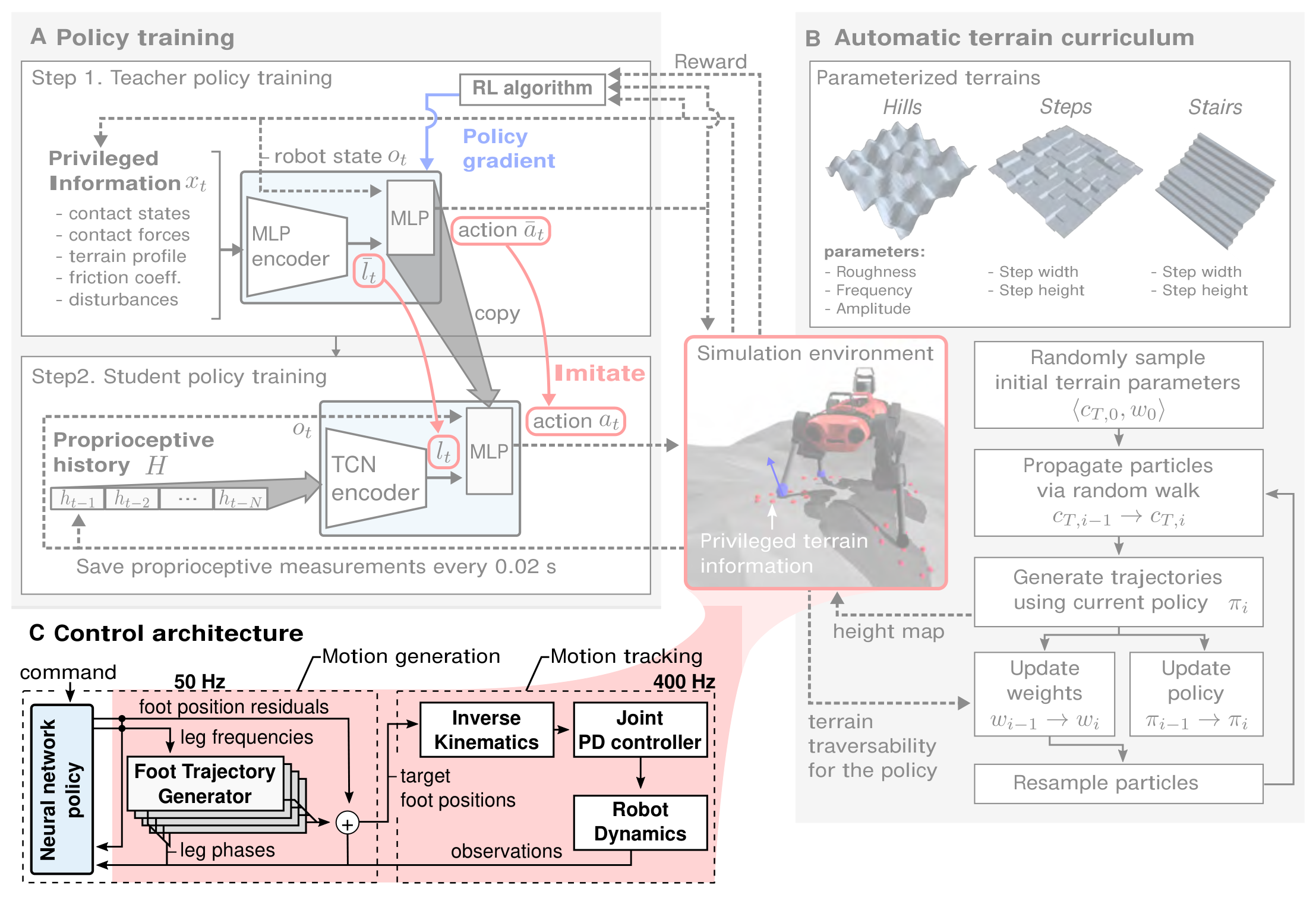
Fig. 4 (p. 7), panel C highlighted. Motion generation at 50 Hz: the policy emits leg frequencies and foot position residuals; four foot trajectory generators turn phases into nominal foot positions; the sum is the target. Motion tracking at 400 Hz: inverse kinematics, joint PD control, robot dynamics. The observations return to the policy.
The action is a 16-vector (p. 8):
| Component | Dimension | What it changes |
|---|---|---|
| leg frequency offsets , | 4 | how fast each leg's phase advances; the base frequency is fixed |
| foot position residuals | added to the generator's output in the horizontal frame |
The data flow from action to torque, with the dimensions that Table S4 and the text give (numbers in parentheses are vector sizes):
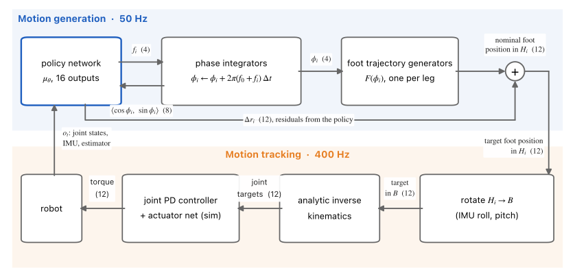
From the 16 policy outputs to torque. Top band, 50 Hz: the four frequency offsets advance the leg phases, the generators turn phases into nominal foot positions, and the twelve residuals are added. Bottom band, 400 Hz: the target is rotated from into the base frame, inverse kinematics gives joint targets, and joint PD control tracks them. Two feedback paths return to the policy: the phases as and the proprioceptive observation .
p.8 · The phase variable, and why it is fed back as cosine and sine
Each leg carries a phase . The first half, , is the contact phase; the second half, , is the swing phase. The phase advances at a rate set by a common base frequency plus the policy's per-leg offset,
as printed on p. 8. Read as the rate at which the phase advances; the printed formula omits the that would convert hertz to radians per second, and the structure is what matters. The base frequency is the trot frequency of the lab's earlier model-based controller (ref. 26), which is where a sensible prior comes from in practice: from the controller you already have.
You have built this object. The GaitScheduler in Convex MPC Biped (My Article) is a phase per side, with a half-cycle offset between legs.
Two differences here. The phase rate is a policy output, so the network can speed one leg up or slow it down, which lets it retime individual legs without a gait library. And the phase does not command contact: in the MPC the phase determined the contact schedule handed to the QP, whereas here the contact half is merely where the generator holds the foot at its lowest point, and contact is a consequence of that geometry. The paper words it as a wish, not a constraint: the legs should "engage ground contact in contact phase" (p. 8).
The phase enters the policy's input as rather than as (p. 8, Table S4: eight numbers for four legs). The reason is a discontinuity that is not physical. The leg's state is continuous through the end of a cycle, but the number jumps from almost to . A network fed the raw angle sees two nearly identical situations as maximally different inputs, and has to learn that and mean the same thing.
The pair is continuous in and one-to-one onto the unit circle, so the same leg state always produces the same input and neighbouring leg states produce neighbouring inputs. This is the standard way to hand an angle to a network; the paper's phrase for it is "a smooth and unique representation for the angle."
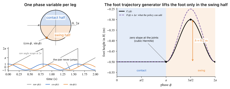
Left: one phase per leg, the contact and swing halves, and why the pair is fed to the network while the raw angle is not. Right: the vertical foot target produced by the generator over one cycle (S3, eq. 11), with the residual the policy can add.
When the operator gives the zero command for half a second, is set to : the phases stop advancing, the generators hold the feet down, and the robot stands still. It restarts at when a direction command arrives or when the base is pushed faster than (S2). This small state machine lives inside the training environment, so the policy learns to stand and to walk under the same controller.
S3 · The foot trajectory generator
The generator is a function from phase to a nominal foot position in the horizontal frame . The supplement's eq. (11) gives only a vertical component, along :
Read it in three pieces.
- During the contact half () the generator holds the foot at its lowest value, along as printed, the stance height.
- During the first half of swing () it rises along a cubic to .
- During the second half () it descends along a second cubic back to .
Each cubic is a Hermite segment with zero slope at both ends, so the foot leaves the ground and lands with zero vertical velocity. That is the same reason the swing-foot planners in model-based stacks use splines with zero end velocity: a soft touchdown does not depend on knowing exactly where the ground is. The paper notes that a sine would also do; any smooth bump works as a prior.
The generator has no horizontal component. The nominal motion is stepping in place, directly under the hip. All forward progress comes from the residuals. The policy is not correcting a walking motion; it is turning a stepping motion into walking by adding lateral offsets that the generator knows nothing about. This is why the residuals are 12-dimensional and the frequencies are the only other output: the generator supplies timing and clearance, the policy supplies placement.
p.8 · The horizontal frame
The generator's output and the residuals are expressed in a frame attached under the hip of leg at the nominal reach. Its -axis is parallel to the gravity vector and its -axis is the projection of the base's -axis onto the horizontal plane. So turns with the robot's yaw but ignores its roll and pitch (p. 8, from Barasuol et al. 2013).
The nominal reach is the leg's hip-to-foot distance in the default standing configuration, not the fully extended length, so the origin of sits at the default foothold of leg : a zero residual leaves the foot where it rests in stance. The origin, though, does none of the work this section credits to the frame. Only the orientation gives the level prior, and a constant translation of the origin is indistinguishable from a constant bias in the residual, which training absorbs; the inverse kinematics needs the hip's position in the base frame in any case. What the choice buys is an action space in which zero means neutral and, because the frame is per-leg, the same residual means the same displacement on all four legs.
Why this matters is easiest to see by imagining the alternative. If foot targets were expressed in the base frame, a pitched base would drag the nominal stepping motion with it: the generator would push feet into the ground on one side and lift them into the air on the other whenever the body tilted, and the policy would have to cancel the tilt with residuals before it could do anything else.
In the prior stays level no matter what the base does, so the residuals only have to handle terrain. The paper's summary is that the frame "reduces the effect of base attitude on the foot motions and consequently stabilizes training" (p. 8).
You have used this frame under another name. The convex MPC of Di Carlo 2018 and the foothold planner in your article both rotate by yaw only, , and treat roll and pitch as disturbances to be corrected rather than as part of the reference geometry (Convex MPC for Legged Locomotion). is the same choice applied to foot targets.
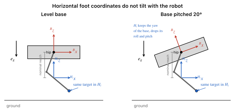
A level base and a pitched base. The base frame (red) tilts with the body; the horizontal frame (blue) keeps only the yaw, so the same target coordinates in put the foot at the same place relative to the ground.
The bracket is the paper's nominal reach: the hip-to-foot distance in the default standing configuration, not the fully extended leg. The origin of is at its lower end, so in stance the foot is at the origin. The figure draws the foot below the origin instead, copying eq. (11) literally; that is the one thing in it not to read as a distance.
Two consequences the paper draws from the frame.
- Converting a target from to the base frame requires the roll and pitch of the base, which is exactly the information the IMU's gravity vector provides (Sensors vs Simulator in Robot RL); yaw is not needed, and the IMU cannot give it anyway.
- Because is aligned with gravity, "lateral" and "vertical" are separate coordinates of the residual, and the stochastic policy's exploration noise can be shaped per direction: larger noise laterally, "to promote exploration along the ground surface" (p. 8).
That sentence is only meaningful once you know that the exploration noise of a Gaussian policy is a standard deviation per action coordinate, which is where §2 begins.
p.8 · Analytic inverse kinematics
Each target foot position is expressed in , rotated into the base frame, and converted to three joint angles by closed-form inverse kinematics. Those joint targets are then tracked by the joint PD controllers at (Fig. 4C), through the actuator net in simulation and the real actuators on the robot.
An ANYmal leg has three joints: hip abduction/adduction (HAA), hip flexion/extension (HFE), and knee flexion/extension (KFE). The inverse problem decouples into two planar problems. In the frontal plane, the lateral offset of the target fixes the HAA angle by a single arctangent. In the plane of the leg, the remaining two joints form a two-link chain, and the law of cosines gives the knee angle from the hip-to-foot distance ; the hip pitch follows from the direction of the target and the interior angle at the hip. Two configurations satisfy the same target, knee forward and knee backward, and the implementation fixes one.
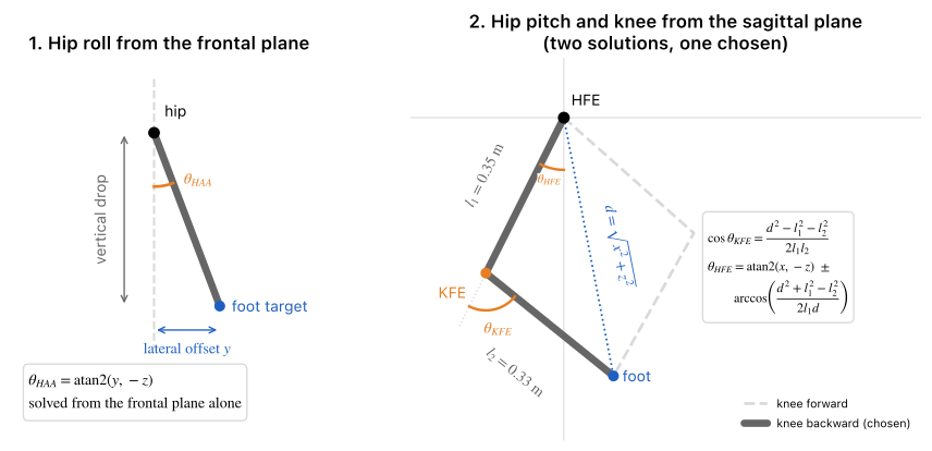
Textbook version of the leg's inverse kinematics. Left: the hip roll angle from the frontal plane. Right: hip pitch and knee angle from the sagittal plane, with the second solution dashed. The real ANYmal leg has a few fixed offsets between joint axes that add terms but not ideas.
The paper gives two reasons for analytic rather than numerical inverse kinematics (p. 8): computational efficiency, since the tracking loop runs at on an onboard CPU, and "to reuse existing position control actuator models for the sim-to-real transfer." The second reason is the deeper one. The actuator net of Hwangbo 2019 was trained on position-control data: joint position error and velocity in, torque out. By ending in joint position targets, this paper reuses the entire tracking stack, the PD law and the learned actuator, without touching it. Whatever the network does upstream, the part of the system that had been validated against hardware stays as it was.
There is also a reason not to skip the foot-space detour and let the network output joint targets directly, and it is the same reason the prior exists at all. Write the leg's forward kinematics as , the foot position as a function of the three joint angles, and differentiate:
Everything follows from the argument of : the request in foot space is a constant, the answer in joint space is configuration-dependent. "Lift the foot two centimetres" is whatever the leg happens to be doing, while the that delivers it is a different triple of numbers for every — small with the leg crouched, large near full extension, where is ill-conditioned in the vertical direction.
So there is no fixed map from phase to joint angles that means "a swing": the same joint trajectory would trace a different foot path every time the posture changed. That is why eq. (11) can be one cubic in one coordinate, and why the per-direction exploration noise of p.8 · The horizontal frame is definable at all — joint space has no axis called lateral. The generator and the network work in the space where the geometry is trivial, and the conversion is charged to the inverse kinematics once per step.
> [!question] Where is a joint angle measured from, and why may it be negative? → Joint Angle Conventions
The Jacobian above is the argument, not the algorithm. Analytic IK inverts in closed form, by the arctangent and the law of cosines of the figure, and never forms ; it is numerical IK that would iterate on , and that is the option p. 8 declines.
2 · Teacher: from policy gradient to TRPO
🔴 for Gaussian policies and the trust-region idea · 🟡 for natural gradient and conjugate gradient (recognise the knobs in Table S7; the derivation is lookup)
This chapter assumes Lecture 7 · Policy Gradient. What it uses from there, and where:
| From L7 | Used here for |
|---|---|
| the objective and its state-distribution convention (L7 §3) | the surrogate objective's expectation over the old policy's states |
| score function and the Gaussian policy (L7 §5) | exploration noise as a standard deviation; the Fisher information matrix |
| policy gradient theorem, advantage, baseline (L7 §6, §8) | the gradient that TRPO follows |
| natural policy gradient, skipped in the video (L7, Gaps) | the direction that TRPO actually steps along |
p.8 · The MDP paragraph, and what off-the-shelf hides
The paper's MDP paragraph is the textbook definition (Markov Decision Process (MDP)): state space, action space, reward, transition probability, a policy , and the discounted return over an infinite horizon. The one non-standard move is the state, : the robot-measurable observation together with the privileged information. With included, the teacher's environment is treated as fully observable, and the paper then says it uses "an off-the-shelf RL method [36]" (p. 8), which is TRPO.
"Off-the-shelf" hides three choices that Table S7 exposes: how the policy is parameterised for continuous actions, how the step size is controlled, and how the constrained step is computed. Each is a prerequisite for reading that table.
Gaussian policies: exploration is a standard deviation
For a continuous action, the standard policy class is a Gaussian whose mean is the network output,
The network computes , a 16-vector of frequencies and residuals. The standard deviations are separate parameters, learned or scheduled, one per action coordinate. Sampling during training is the exploration; at deployment the mean is used and the controller is deterministic. The score function for the mean is , which is L7's Gaussian policy slide (Lecture 7 · Policy Gradient › p.17–18 · Softmax and Gaussian Policies ⏱ 36:49): actions that came out above the mean and turned out well push the mean up.
Now the sentence from §1 reads plainly. "We applied larger noise in the lateral direction" (p. 8) means is larger for the and components of the residuals than for . That is only a well-defined choice because the residuals live in , where is along gravity. The stated aim is "to promote exploration along the ground surface" (p. 8): lateral exploration tries different footholds, which is where the terrain problem lives.
Why a step size in parameter space is the wrong knob
Vanilla policy gradient updates with a learning rate measured in parameter space. The problem is that the same can be a negligible or a catastrophic change in behaviour, depending on where the policy currently is.
The Gaussian makes this concrete. Shift the mean of by . The Kullback–Leibler divergence between old and new policy is
so the same parameter step is a divergence of when and of when . In the second case almost every action the new policy samples would have been essentially impossible under the old one. As training narrows , a fixed learning rate turns into ever larger policy changes, exactly when the policy has become good and has the most to lose.
Two things go wrong when a step changes the policy too much. The gradient estimate was computed from the old policy's data and is a local statement; far from it says nothing, so the step may make things worse. And a locomotion policy that has been made worse generates worse data (short episodes, falls), from which recovery is slow. This is the failure people call performance collapse, and avoiding it is the entire motivation for measuring the step in the space of behaviours rather than of parameters.
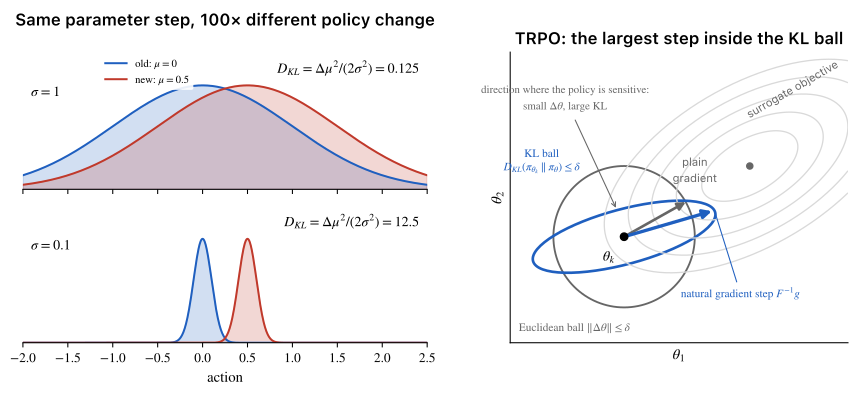
Left: the same mean shift is a small or a huge change of the action distribution depending on . Right: in parameter space, a ball of constant KL divergence is an ellipse whose shape depends on the current policy; TRPO takes the largest step inside it, which is the natural-gradient direction .
The TRPO problem and its guarantee
TRPO (Schulman et al. 2015) replaces the learning rate by a constraint. Let be the current parameters and the state distribution the current policy visits. The surrogate objective is
and the update is the solution of
Three things to see in the surrogate.
- The ratio is an importance weight: the actions were sampled from the old policy, and the ratio re-weights them to evaluate the new one, exactly the one-step ratio of Importance Sampling in Off-Policy RL.
- The states, by contrast, are not re-weighted; they stay distributed as under the old policy, which is an approximation that is accurate only while the two policies are close.
- At the ratio is , so (the advantage has zero mean) and , the policy gradient of L7.
To first order the surrogate is the L7 objective; it differs in how far from it is trusted.
The reason to trust it inside a KL ball is a theorem (Schulman et al. 2015, Theorem 1, building on Kakade and Langford 2002). For any two policies,
where is the largest per-state divergence. The right-hand side equals at . So maximising the right-hand side and moving to its maximiser can never lower : it is a lower bound that touches the objective at the current point, and pushing the bound up pushes the objective up with it. This argument, maximise a touching lower bound, is the minorisation–maximisation pattern, and it is the correctness bridge between the surrogate and the true return.
Two approximations separate the theorem from the algorithm, and both are worth stating precisely because the guarantee does not survive them unchanged. The penalty coefficient is enormous for near , so maximising the penalised bound would produce steps too small to be useful; TRPO therefore replaces the penalty by the hard constraint with a tuned hyperparameter. And the theorem's over all states cannot be estimated from samples, so the constraint uses the mean KL over visited states instead. With those two substitutions the monotonic-improvement guarantee becomes a heuristic that works well in practice, not a theorem.
From the constrained problem to the update rule
The constrained problem cannot be solved exactly for a network with on the order of parameters (the student networks in Table S6 have about ; the teacher is of the same order), so TRPO solves a local approximation of it and then checks the result.
Linearise the objective and quadratise the constraint around :
where is the policy gradient estimate and is the Hessian of the mean KL at , which is the Fisher information matrix . The first-order objective under a quadratic constraint has a closed-form maximiser:
The direction is the natural gradient of L7's skipped slides (Lecture 7 · Policy Gradient › Gaps to close on your own): the steepest direction when distance is measured by KL rather than by the Euclidean norm on . The scalar in front is the step length that lands exactly on the boundary under the quadratic approximation.
The obstacle is . For parameters it has entries; it can be neither stored nor inverted.
TRPO never forms it. It solves with the conjugate gradient method, which only needs the product for a given vector , and that product is available by automatic differentiation of the KL at the cost of a few backward passes per iteration. A small multiple of the identity is added, , so that the system is well-posed when is nearly singular; this is the "CG damping" of Table S7. Ten to fifty iterations give a good enough .
Finally, because both approximations can be off, the full step is checked against the real quantities: a backtracking line search shrinks by a constant factor until the sampled mean KL is at most and the sampled surrogate has actually improved. That check is what makes the method robust in practice: the approximations propose, the constraint decides.
The theorem bounds the true return using the maximum per-state KL; the algorithm constrains the mean. The theorem's penalty is replaced by a constraint whose is tuned. The Fisher matrix is estimated from the same batch as the gradient. Each of these is standard, and each is a place where the guarantee is no longer a guarantee. When a later paper says its clipping "approximates a trust region", the Paper Reading Roadmap already lists the paper that checks whether it does (Engstrom et al. 2020, Section 5).
Reading Table S7
With the pieces above, Table S7 is a list of knobs on this algorithm, not a list of numbers to remember.
| Row | What it is |
|---|---|
| discount factor | the effective horizon policy steps, at the of Fig. 4C |
| KL-d threshold | , the radius of the trust region in mean KL |
| max. episode length | at per step, unless a fall terminates earlier |
| CG damping | in |
| CG iteration | conjugate-gradient iterations used to approximate |
| batch size | state–action samples collected per policy update, from parallel simulations |
| total iterations | policy updates; with the batch size, about simulated steps for the teacher |
S4 · Reward: what changed since Hwangbo 2019
The reward is the seven-term sum of S4. The pattern from Bounded Kernel Rewards in Robot RL holds: objective terms are bounded, penalty terms are unbounded norms. What is new is worth listing because it is easy to read past.
| Term (S4) | Role | Needs, and from where |
|---|---|---|
| linear velocity | objective: progress along the command | , the base velocity projected on the commanded direction; estimator |
| angular velocity | objective when a turn is commanded | yaw rate; IMU |
| base motion | bounded term, largest when the velocity orthogonal to the command and the roll and pitch rates are zero | estimator and IMU |
| foot clearance | bounded term: the fraction of swing feet higher than the scanned terrain around them | the height scan around each foot: privileged, simulator only |
| body collision | penalty: minus the number of body contacts other than feet | contact set: simulator only |
| target smoothness | penalty: minus the norm of the second finite difference of the foot targets | the two previous targets, which is why they are in |
| torque | penalty: minus the norm of the joint torques | actuator net in simulation |
Three differences from Hwangbo 2019.
- The paper maximises a reward instead of minimising a cost, and the penalty terms carry their minus sign inside their own definitions (eqs. 16–18: , and likewise for smoothness and torque), so every coefficient in the sum is positive and there is no sign puzzle of the kind Hwangbo's S3 had.
- The objective term is capped rather than bell-shaped: for and above it (eq. 12), a one-sided kernel that rewards approaching the cap and stops caring beyond it; the cap is the top speed of the model-based controller the lab had before (ref. 26).
- There is no curriculum factor on the penalties; the curriculum in this paper acts on the terrain, which is §5.
The two rows marked simulator-only are the observation-versus-cost split of Sensors vs Simulator in Robot RL at work: the reward may use a height scan the robot will never have, because the reward is only ever evaluated in simulation.
3 · Privileged learning: teacher, student, and DAgger
🔴
p.3, p.6 · The problem: one scalar per step cannot teach two things
The paper reports (p. 3) that training the proprioceptive network directly by RL failed: "the supervisory signal was sparse and the presented network failed to learn locomotion within reasonable time budgets." The ablation in Fig. 5E–G shows the same thing under controlled conditions: a TCN-20 trained by TRPO on proprioception alone, with the teacher's reward and hyperparameters, never learns to balance (short episodes, low reward), while the same architecture trained by imitation of a privileged teacher does.
Read "sparse" as a statement about how much the signal says, not about how often it arrives; a reward arrives every step. This reading is mine, not the paper's, but it is what the ablation supports.
One scalar per step, mixing seven objectives, has to teach a network both what to extract from a two-second history (is a foot trapped? is the ground sloping? was I pushed?) and what to do about it. The two problems are coupled: the network cannot learn what to extract until it knows what matters for acting, and cannot learn to act well until it extracts the right things. Privileged learning breaks the coupling by solving the second problem first, with the answer to the first handed over as input.
The pattern comes from learning by cheating (Chen et al. 2019), where an agent with access to the ground-truth layout of a driving scene is trained first, and a second agent that sees only camera images is trained to imitate it. This paper's variation is that the privileged agent is trained by RL rather than from human demonstrations, because nobody can demonstrate ANYmal over rough terrain.
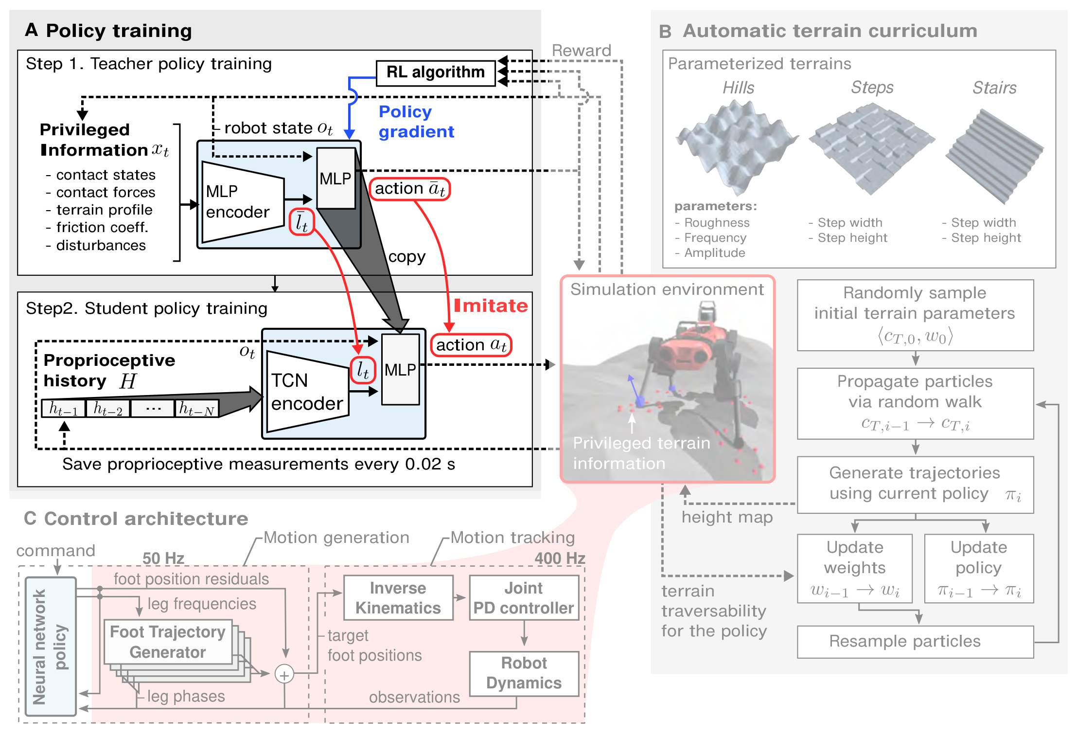
Fig. 4 (p. 7), panel A highlighted. Step 1: the teacher is trained by policy gradient with the privileged information as part of its input. Step 2: the student, with a proprioceptive history in place of , is trained to reproduce both the teacher's latent and its action . The head layers are copied.
p.8 · Privileged information: what the teacher is allowed to know
Table S4 lists the privileged block : the terrain normal at each foot, the elevation of nine scan points on a circle around each foot, foot contact forces and states, thigh and shank contact states, the friction coefficient under each foot, and the external force applied to the base during training. Every one of these is a hidden cause of something the student will see in proprioception: a slipping foot, an unexpected stop of a descending leg, a base that accelerates without the legs having done anything.
The rule of Sensors vs Simulator in Robot RL is that an observation must be measurable on the robot. That rule was stated for a policy that deploys. The teacher does not deploy, so its observation may contain simulator-only quantities, exactly as the reward always could. The split between what is allowed in the reward and what is allowed in the observation has moved: for the teacher, both lists are the simulator's.
The teacher does not consume raw. An encoder compresses it into a 64-dimensional latent (Table S5: ), and the action head takes together with . The command and the robot's own state are deliberately kept out of , so that "contains only the terrain- and contact-related features" (p. 8). That bottleneck is a design choice made for the student's sake: it produces a compact, well-defined target for what the student's history must encode, "what the ground is doing", in 64 numbers.
p.9 · Behavior cloning is regression, and where it breaks
Imitation learning in its simplest form is supervised regression. Given a dataset of input–label pairs , where is the expert's action at that input, fit a policy by minimising the squared error over the dataset. The paper's student loss is this, with two labels (eq. 1):
Bars are the teacher's outputs, computed with the privileged ; unbarred are the student's, computed from the history . Compared with RL, this is an easy problem for two reasons. The supervision is dense: eighty numbers per step, sixteen action components and sixty-four latent components, each with a definite target, instead of one scalar. And there is no credit assignment across time: each step is its own regression problem.
The catch is the distribution the regression is accurate on. A regressor is accurate on inputs like those it was trained on. If is collected by running the teacher, the student learns to be accurate on the states the teacher visits.
But the student is not the teacher. Its small errors move it to states slightly off the teacher's distribution, where it was trained less and errs more, which moves it further off, where it errs more still. This is covariate shift, and in sequential decision-making it compounds: Ross and Bagnell (2010) show that a per-step imitation error of on the training distribution can cost over a horizon of steps, because one mistake can put the learner in unfamiliar states for the rest of the episode. Plain behavior cloning of a locomotion teacher would produce a student that walks well for a moment and then falls in ways the teacher never did.
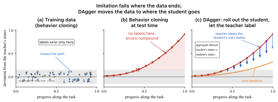
Left: behavior cloning trains only on the teacher's states. Middle: at test time the student's own errors take it where no labels exist, and they compound. Right: DAgger rolls out the student and asks the teacher for labels at the student's own states, so the next student is trained where it actually goes.
p.9 · DAgger: label where the student goes
DAgger, dataset aggregation (Ross, Gordon, and Bagnell 2011), fixes the distribution by changing who generates the states. Iterate: run the current student and record the states it visits; ask the expert for its action at each of those states; add these pairs to the aggregate dataset; retrain the student on everything collected so far. The original algorithm mixes expert and student control in early iterations with a decaying probability ; the essential step is that the labels are collected on the student's state distribution. Under a no-regret learner, the returned policy's cost is plus regret terms rather than (Ross et al. 2011, Section 3, Theorems 3.1–3.2).
The paper's description is one sentence and is exactly this: "training data is generated by rolling out trajectories by the student policy. For each visited state, the teacher policy computes its embedding and action vectors" (p. 9).
Notice what DAgger requires of the expert. It must answer "what would you do here?" at arbitrary states chosen by the student, not just at states on its own trajectories. A dataset of human demonstrations cannot do that. A teacher that runs in the simulator can, trivially: at whatever state the student has reached, the physics engine supplies , the teacher network is evaluated, and the labels are written down. This is the second reason privileged learning and DAgger belong together, and it is another consequence of the tip in The one idea.
Once the student is trained on its own state distribution, there is no shift between training and test in simulation. The remaining shift is between simulation and the robot, and DAgger does nothing about that one. It is addressed, as in Hwangbo 2019, by randomising dynamics and friction, adding observation noise and pushes, and by the actuator net (S2).
p.9, S9 · Why imitate the latent, and why copy the head
Two design details make the student's job easier and are easy to miss.
The action head of the student is not trained from scratch. Table S5 marks the layers output as copied from the teacher after teacher training. If the student's encoder produced exactly, the copied head would produce exactly. So the two loss terms are consistent by construction: the latent term teaches the encoder what to extract from the history, and the action term corrects whatever the latent term leaves. Imitation mostly trains the new part, the encoder.
The latent term matters. S9 ablates it: a student trained on the action term alone ("naive IL") matches on slopes and under pushes but has a lower success rate on steps. The reading is that the action target alone tells the encoder only what is needed to reproduce actions on the training distribution, while the latent target says explicitly which sixty-four features about the ground to recover, a denser and more direct supervision of the representation.
| RL from scratch (Fig. 5E–G baseline) | Behavior cloning | DAgger (this paper) | |
|---|---|---|---|
| who generates the states | the learner | the teacher | the learner |
| who provides the targets | the reward, one scalar per step | the teacher, on the teacher's states | the teacher, on the learner's states |
| signal per step | 1 number, mixed objectives | 80 numbers | 80 numbers |
| needs the teacher at test time | no | no | no |
| fails when | the two coupled problems are too hard for the reward to separate | the learner leaves the teacher's distribution | the learner's input cannot carry what the teacher knew |
The last cell is the student's real ceiling. It can only recover what the history predicts. Terrain that has not yet been touched leaves no trace in proprioception, which is why the paper's Discussion calls the gait "fairly conservative since it must by necessity feel out the environment with its body as it locomotes" (p. 6), and why the paper points to a hybrid proprioceptive–exteroceptive controller as future work.
4 · Memory: partial observability and the TCN
🔴 for the partial-observability argument and causal 1-D convolution · ⚪ for the recurrent alternative
p.8–9 · Why the student needs a history
The student sees and not . Everything in still affects what happens next, so the student's observation is not a Markov state: the same can occur with a foot about to hit a step or on flat ground, on ice or on rubber, pushed or not pushed.
In RL vocabulary the student faces a partially observable problem, a POMDP (Silver L1; the POMDP slides of L2 were skipped, but the aliased gridworld of Lecture 7 · Policy Gradient › p.7–9 · Aliased Gridworld ⏱ 15:25 is the same failure in miniature: identical observations in different situations). A policy that reacts to alone must react identically in situations that call for different actions.
There are three standard cures.
- The exact one: the belief state, the posterior over the hidden variables given the whole history, which converts the POMDP into an MDP over beliefs; it is exact and intractable here.
- The second: feed a window of recent observations and let the network compute whatever statistic of it is useful.
- The third: a recurrent network that carries a state forward.
The paper takes the second cure with a window of observations at , two seconds, and states its hypothesis on p. 8: the teacher's latent "can be (partially) recovered from a time series of proprioceptive observations." The word partially is honest: the history predicts what has been touched, not what lies ahead.
Why should hidden causes be recoverable from proprioception at all? Because they leave traces.
- A foot that hits a step stops descending early: a jump in position error and a drop in velocity in that leg's joints.
- A foot that slips moves while the leg is in stance.
- A push changes the base velocity without any leg having done anything to cause it.
- Terrain height is where the foot stopped.
Hwangbo 2019 already exploited this with a history of two samples, as its substitute for a contact sensor (Sensors vs Simulator in Robot RL › Contact detection without a force sensor); this paper extends the same idea to a hundred samples and lets the network decide what to extract.
How much history is needed is an empirical question, and the paper answers it in Fig. 5B–D. On a uniform slope, one sample is enough; the slope is visible in the gravity vector at every instant. On a step, memory decides: the hind legs have to clear a step that only the front legs have touched, a second or more earlier at walking speed, and short-memory controllers fail there. Under a lateral push, the two-second controller deviates about a third less than the one-sample controller.
Three quantities are dropped from the student's per-step input (p. 9): the base frequency, the joint history, and the previous foot targets. All three were short-hand histories inside , and they are redundant once the window itself is the input.
The DSP view: a causal 1-D convolution is an FIR filter with learned taps
The student's encoder is a temporal convolutional network, TCN (Bai, Kolter, and Koltun 2018). You know its building block under another name. A one-dimensional convolution over time with filter size ,
is a finite impulse response filter: taps, applied to the current and past samples, the same taps at every . The only difference from Signals & Systems is that the taps are learned by gradient descent rather than designed. With many input channels (the proprioceptive signals of ) and many output channels, each output channel is a sum over input channels of such filters: a filter bank with channel mixing. A ReLU after each layer makes the stack nonlinear, so the whole network is not an LTI system, but each layer's linear part is.
| Signals & Systems | Convolutional network |
|---|---|
| impulse response, taps | kernel, weights (learned) |
| causal filter: uses , only | causal convolution |
| filter length | filter size, here |
| sparse taps at spacing | dilation |
| decimation by | stride |
| filter bank, channels | input and output channels |
| cascade of filters with pointwise nonlinearities | stacked layers with ReLU |
| the span of input samples a filter output depends on | receptive field |
Three adjectives in the paper's one-sentence description of the encoder (p. 9) now have precise meanings. Causal: the output at uses no samples after , which is what makes the network runnable in real time, one output per new sample. Dilated: a layer with dilation places its taps samples apart, , so that stacking dilations multiplies the span the output sees while the number of taps grows only linearly. Strided: a stride- layer keeps every second output, which is decimation by two; the sequence gets shorter and the layers after it cheaper.
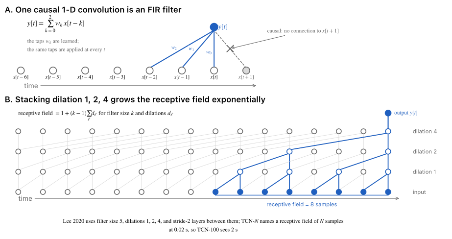
Top: one causal 1-D convolution is an FIR filter whose taps are learned. Bottom: stacking layers with dilations 1, 2, 4 grows the span of the input the final output can see; only the blue connections feed that output.
For a stack of layers with filter size and dilations , all with stride , the receptive field is
A stride- layer doubles the input spacing of every layer after it, so the same formula applies with each later multiplied by the accumulated stride.
Table S5 · TCN-N, and what the ablation held fixed
The student encoder in Table S5, filter size , ReLU after each convolution:
| Layer | Type | What it does to the window |
|---|---|---|
| 1 | 1-D conv, dilation 1 | local FIR over consecutive samples |
| 2 | 1-D conv, stride 2 | decimate: |
| 3 | 1-D conv, dilation 2 | taps samples apart at the decimated rate |
| 4 | 1-D conv, stride 2 | decimate again |
| 5 | 1-D conv, dilation 4 | taps samples apart |
| 6 | 1-D conv, stride 2 | decimate again |
| 7 | the latent that must match | |
| 8 | concatenate with | the current observation joins the summary of the past |
| 9–12 | output | the head copied from the teacher |
Working the receptive field through these six layers with the formula above (my computation from Table S5, tracking the accumulated stride) gives a span of about input samples for the last output, so with the final output sees the whole two-second window. TCN- in the paper denotes a receptive field of time steps (p. 12), realised by feeding a window of observations: TCN-1 sees , TCN-20 sees , TCN-100 sees .
One detail in Table S6 makes the memory ablation a fair one. The channel counts differ, , , for TCN-1, TCN-20, TCN-100, and they were chosen so that all three networks have about parameters. The comparison in Fig. 5B–D therefore isolates history length; it is not confounded by capacity. The cost of memory shows up instead as training time: one gradient update takes about for TCN-1 and for TCN-100.
S8 · The recurrent alternative, as an anchor
A gated recurrent unit keeps a state, , that in principle summarises the entire past; in filter language it is closer to an IIR recursion than to an FIR window. It is trained by backpropagation through time, and truncated BPTT limits how far back the gradient is propagated, for cost and stability. The paper's GRU student (S8, Fig. S3) lands between TCN-20 and TCN-100 in performance and takes three times longer per update than TCN-100 (Table S6), because a recurrence must be computed sequentially while a convolution over a window is computed in parallel across time.
The paper's stated reasons for choosing the TCN are the ones you can now read: transparent control over the history length, long histories, and robustness to hyperparameter settings.
5 · Curriculum: from Bayes filter to particle filter
🔴 for this paper · 🟡 in general, since the same filter returns in robot state estimation
The probability, Bayes-filter, importance-sampling, and resampling mathematics under this chapter is taught in Bayes and Particle Filters (in Korean); here each such step gets a sentence or two and a link to the lecture section that teaches it.
p.9, p.12 · The problem: which terrains to train on, and what uniform sampling costs
Every training terrain is generated from a terrain parameter vector , and during training "the terrain is regenerated every episode with a different random seed" (S5, p. 16). The generators are in S5 and the bounds of in Table S2 (p. 20):
| Terrain | Generator (S5) | and range (Table S2) | Friction coefficient | Grid size (Table S2) |
|---|---|---|---|---|
| Hills | Perlin noise plus uniform noise, | roughness , frequency , amplitude | ||
| Slippery Hills | Hills with lower friction | as Hills | ||
| Steps | square steps: for every block, a height drawn from | step width , step height | ||
| Stairs | a staircase with fixed step width and height; the robot starts on the flat middle segment | step width , step height |
is a Gaussian with mean and standard deviation , clipped above ; the unit of frequency is not given. S5 names three generators, and the ablation on p. 12 names hills, steps, and stairs as the training terrains. The ranges were chosen "considering the kinematics of the robot" (S5), for example a step height below the leg length.
The curriculum decides which the policy trains on at each point of training. The paper applies it during both teacher and student training (p. 8), but Algorithm S1 and the ablation on p. 12 describe teacher training only.
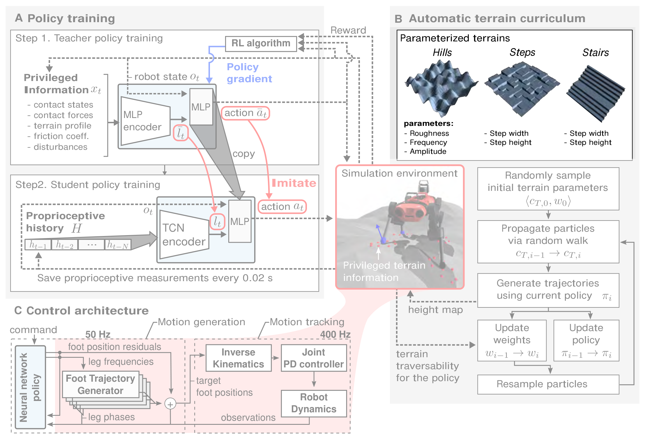
Fig. 4 (p. 7), the terrain box of panel B highlighted. Hills with roughness, frequency, and amplitude; Steps and Stairs with step width and step height. Slippery Hills, the fourth row of Table S2, is not drawn.
The baseline is the obvious one: a teacher trained on terrains sampled uniformly from as specified in Table S2 (p. 12, Fig. 5H–J). Without the curriculum the success rates on the test terrains are significantly lower (5H), the reward plateaus at a lower level (5I), and the mean episode length is shorter throughout training (5J). Each model was trained with five random seeds and the error bars are 95 % confidence intervals (Fig. 5 caption, p. 10), which is how to read the comparison (§6).
The paper attaches its explanation to the shorter episodes (5J): uniform sampling more often draws terrains the policy being trained cannot traverse, and on those the policy "fails early and receives less training signal as a result" (p. 12). Its summary is that the adaptive curriculum modulates terrain difficulty "so as to maximize the didactic benefit of each episode."
That explanation covers only the hard side. The upper threshold introduced below also excludes terrains that are too easy, but the paper gives no training-signal argument for that side, and p. 12 does not test it. Treat "easy terrains teach little too" as an interpretation.
Two things are both called a curriculum in the papers you are reading, and they are different objects.
| Hwangbo 2019, cost curriculum | Lee 2020, terrain curriculum | |
|---|---|---|
| what is scheduled | the weight of penalty terms in the cost | the distribution the training terrains are drawn from |
| driven by | a fixed schedule over training iterations | the current policy's measured traversability on each particle's terrain |
| purpose | let the task be learned before the constraints bite | "maximize the didactic benefit of each episode" (p. 12) |
| where it acts | inside the reward | in the environment generator; the reward is unchanged |
The paper places itself among automatic curriculum learning methods for RL agents (p. 9). POET generates parameterised terrains for a 2D bipedal agent and uses minimal criteria to choose environment parameters that are neither too challenging nor trivial, realised by selecting parameters that yield mid-range rewards; Florensa et al. similarly choose achievable yet difficult goals. The paper states one difference from POET directly, the aim: POET runs an open-ended search and evolves a population of specialised agents, while this paper wants a single generalist agent. A second contrast follows a paragraph later, where POET is among the methods that use the reward function to evaluate learning progress [25, 41–43], while this paper evaluates by traversability (next subsection).
p.9 · Traversability and desirability: hard but passable as probabilities
Traversability is defined as "the success rate of traversing a terrain" (p. 9). The paper's only reason for using it instead of the reward is that it found traversability "more intuitive than the reward function", which consists of multiple objectives that are often unbounded (p. 9).
The ingredient is a label on each state transition (eq. 2),
where is the inner product of the base velocity and the commanded direction at step , horizontal components only (S4; notation in Appendix B). Both inequalities are strict as printed, so the case is assigned to neither line. The threshold, in , is a hyperparameter, "about one third of the maximum speed of our robot" (p. 9); S4 gives that maximum as on flat terrain with the lab's earlier controller.
Traversability is the expectation of that label (eq. 3),
with the trajectories generated by , following a definition of empirical traversability in prior work (ref. 44). What you need here is one fact: the expectation of an indicator is a probability, which is why lies in and reads as a success rate. The symbol is not a matrix trace.
The objective is terrains with mid-range traversability, and the rationale is to synthesise terrains that are "neither too easy nor too difficult" (p. 9). Desirability is defined as (eqs. 4–5)
where and are fixed minimum and maximum thresholds. The indicator is missing from eq. 5 as printed (p. 9); it is restored here from eqs. 7 and 10.
The inside the probability is the traversability of a single trajectory, a random quantity; is the probability that it lands in the band. Read against eq. 3 alone, is one number and could only be or . Eq. 5 takes the expectation over , and eq. 7 below counts trajectories, so the indicator is applied trajectory by trajectory. The paper does not write the single-trajectory out; the reading consistent with eq. 3 is the fraction of that trajectory's transitions with . It also does not say why it thresholds each trajectory rather than the pooled rate.
What makes two trajectories on the same differ is not discussed as such. The ingredients are all in the paper: a random initial position (Algorithm S1, line 7), a new terrain seed each episode (S5), and randomised dynamics, disturbances, and observation noise (S2).
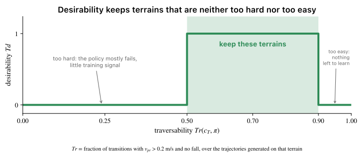
The curve is the indicator as a function of a traversability value, although the vertical axis is labelled . Desirability is the probability that this indicator equals for a trajectory (eqs. 4–5), so it can take any value in . Two labels are the figure's, not the paper's: "nothing left to learn" on the easy side, and the footnote's pooling of transitions over all trajectories, whereas eq. 7 applies the indicator to each trajectory's .
Desirability becomes a measurement model through a binary variable (p. 9): if . Then (eq. 6)
The middle term is printed with , a typo for . What you need is a two-valued measurement model and the likelihood: read with varying, is the likelihood of , not a distribution over . Only this value is ever computed (eq. 6, Algorithm S1 line 14); no enters a weight.
In practice the measurement probability is the empirical expectation over the samples collected during policy training (eq. 7):
where is the number of trajectories generated using (the sum is printed without a lower index). "The trajectories are also used for policy training," so the curriculum needs no additional evaluation steps (p. 9). S2 then slows the update: the curriculum is updated every policy iterations "to reduce variance," assuming the policy's performance is similar within that window, and the estimate becomes (eq. 10)
is judged per trajectory, and the measurement probability is the in-band fraction pooled over trajectories per particle per curriculum update (Table S3).
How noisy is that fraction? If the 60 in-band indicators were independent Bernoulli trials with a common , their count would be binomial with variance , so the fraction would have standard deviation , at most , against at most from alone. That is my arithmetic, consistent with the direction of the paper's stated reason. The window guarantees neither independence nor a common : the policy is updated ten times inside it, and the paper assumes, rather than shows, that its performance stays similar. Without a common the fraction estimates the window average of rather than for one policy; without independence, since later policies are trained on earlier trajectories, the standard deviation can exceed the bound.
p.9 · What is filtered: the textbook particle filter, piece by piece
The paper says its algorithm is "modeled on the Sequential Importance Resampling (SIR) particle filter" (p. 9). Its target is the distribution of terrain parameters that satisfy , and the set of tuples , , "approximates the target distribution." In the lectures' sense a weighted particle set approximates a distribution when its weighted averages match expectations, not density values point by point.
The tracked quantity is not a hidden physical state. It is a distribution over terrain parameters, concentrated where terrains are desirable for the current policy. It changes during training because has the policy as an argument, not because terrains have dynamics.
| Textbook particle filter | Lee 2020 | Stated in the paper, or my reading | Lecture |
|---|---|---|---|
| target: the posterior over a hidden state given the measurements | the distribution of with | stated (p. 9); that it moves with the policy follows from the definition of | L4 §4 |
| one particle's value | , a terrain parameter vector | stated as a "sampling point" (p. 9); the paper never calls it a state | L5 §5 |
| time step | curriculum iteration , one per policy updates | stated (Algorithm S1 lines 3, 22; S2) | Bayes filter recursion |
| Markov assumption | assumption 3: forms a Markov process | stated (p. 9); see the caveat in the assumptions | L3 §5 |
| transition model , a known model of how the state evolves | random walk to adjacent values with , plus draws from a replay memory with | random walk stated as the transition model (p. 9, line 21); replay draws (line 20, S2) are a separate step, and grouping them with the transition is my reading, as is that the walk is a design choice with no process behind it | L3 §3 · L5 §6 |
| initial belief | uniform over | stated (line 1); the p. 9 text also allows starting concentrated on almost flat terrain | L5 §5 |
| measurement | if | stated (p. 9) | L3 §3 |
| likelihood , evaluated exactly | , estimated by an in-band fraction of 60 trajectories | stated (eqs. 6, 7, 10); no lecture treats an estimated likelihood | L2 §2 |
| weight and normalisation | line 16: each particle's measurement probability over the sum across particles, no previous-weight factor | stated (line 16); why that is consistent is my reading, in Algorithm S1 | L6 §6 · L6 §4 |
| resampling | line 17, with probability for the th sample | stated (p. 9, line 17) | L7 §4 |
| estimate | none; the particles are the terrains of the next rollouts (line 6) | line 6 stated; that no estimate is formed is my reading of Algorithm S1 | L7 §7 · L6 §4 |
| remedies for degeneracy, impoverishment, deprivation | replay memory | purpose stated (S2), mechanism not | L7 §5 · L7 §6 |
The paper never uses the name "bootstrap filter." With the transition as the proposal and resampling in every cycle, Algorithm S1 has the structure the lecture series calls SIR, the bootstrap filter; that match is my reading, and the differences are listed at the end of Algorithm S1.
Why particles at all, when is bounded and discretised and a finite discrete state is one of the cases where the exact recursion is computable? The paper does not discuss it. Its stated reason for bounding and discretising is exploration: "to reduce the search space" (p. 9). One reading, mine: every likelihood value here costs simulated trajectories, and particles spend that budget only at the values they occupy. Table S2 lists a "grid size" per terrain type ( for Hills, for Steps and Stairs) but does not say what it is. A single length per terrain type would have to serve every parameter of that type, including Hills' frequency, whose unit is not given, so on my reading it is more likely the height-map resolution than an increment of . The paper states no increment for explicitly.
p.9 · The three assumptions
The paper lists three assumptions (p. 9) and says where the first comes from and what the second and third are for.
- Terrain parameters with similar are close in Euclidean distance in parameter space. Source: the insight that terrain parameters can be interpolated; for example, a staircase gets harder as the step height increases.
- A policy trained on terrains from some area of learns to interpolate to nearby terrain parameters. Role: it justifies training on discrete samples from for a policy that generalises over a region of ; the paper gives no support for the assumption itself.
- forms a Markov process, where is the particle set at iteration . Role: it "is necessary for formulating a particle filter." Support: the random walk satisfies it because each parameter's evolution depends only on its current value and randomly sampled noise.
Mind the direction of assumption 1: similar traversability implies nearby parameters. It does not say the converse, that nearby parameters have similar traversability. The paper does not link assumption 1 to the random walk; its only support is the interpolation example.
For assumption 3, what you need is the full-form Markov assumption. One caveat is mine, not the paper's: line 20 draws from a replay memory to which each cycle's particle set is appended (line 18; no capacity or eviction rule is stated), so the next set can depend on more than the current set. The process is Markov if the memory is counted as part of the state; the paper's justification mentions only the random walk.
Algorithm S1 · One iteration of sequential importance resampling
Algorithm S1 (p. 15) is titled "Teacher training with automatic terrain curriculum." Condensed, with the paper's line numbers and loop nesting:
 1 init replay memory; N_particle c_T,0 ~ U(C); i, j = 0
 2 repeat
 3   for 0 <= k <= N_evaluate:
 4     for 0 <= l <= N_particle:
 5       for 0 <= m <= N_traj:
 6         generate terrain using c^l_T,j
 7         initialize robot at random position
 8         run policy pi_i
 9         label each state transition (Eq. 2)
10         save the scores and the trajectory
11     update policy using TRPO
12     i = i + 1
13   for 0 <= l <= N_particle:
14     measurement prob. of c^l_T,j (printed Eq. 9)
15   for 0 <= l <= N_particle:
16     update weights (see below)
17   resample N_particle parameters
18   append c_T,j to the replay memory
19   for 0 <= l <= N_particle:
20     w.p. p_replay: sample from replay memory
21     w.p. p_transition: move c^l_T,j to adjacent value
22   j = j + 1
23 until convergence
Table S3 (p. 20) sets per terrain type, , , , and (capital in the table, lower case in line 20). The loop bounds are printed inclusively, , which read literally would give iterations while eq. 10 divides by ; the paper does not comment, so read each loop as running exactly its bound's number of times (, , ), which for and is what eq. 10's divisor requires.
Two counters run at different rates: counts policy updates (line 12), counts curriculum updates (line 22). One curriculum update spans policy updates.
Lines 3–12 are ordinary teacher training. For each particle, episodes are run on terrains generated from that particle's value, each with the robot at a random position, and every transition is labelled by eq. 2. The TRPO update of §2 sits inside the loop, after the rollouts of all particles, so each policy update consumes trajectories from every particle's terrain. That is the paper's "no additional evaluation steps": the rollouts that train the policy are the ones the curriculum scores. Table S3 counts 10 particles per terrain type; the paper does not say whether the types form separate filters or how their rollouts are combined into one TRPO batch. The window of policy updates exists "to reduce variance," under the assumption that the policy's performance is similar within it (S2).
Lines 13–14 compute each particle's measurement probability. The printed reference "Eq. 9" is a typo: eq. 9 is the saliency map on p. 12, and the formula that pools over and , matching these loops, is eq. 10.
Lines 15–16 compute the weights, printed as
The weight carries no particle index , and carries the policy counter where eq. 6 writes ; read both as notation slips. What matters is the structure: the weight is recomputed each cycle from the current measurement probability alone, with no previous-weight factor. The normalisation is the sum in the denominator (self-normalisation).
Why that is consistent, which the paper does not explain: line 17 resamples in every cycle, so the particles entering the next weighting carry equal weights. Without resampling the weight would be the product ; after resampling at every step, is absorbed into the proportionality, and the weight is the likelihood under the transition used as the proposal.
The lectures assume the likelihood is evaluated exactly at each particle. Here it is a random fraction, and two consequences have no lecture behind them.
- The weights inherit the estimate's noise. If the policy were fixed over the window, the fraction would be an unbiased, non-negative estimate of ; independence of the trajectories matters for its variance, not its mean. Particle filters that put such estimates into the weights go by the name random-weight particle filters, and the lectures do not cover them.
- A particle whose 60 trajectories all fall outside the band gets weight and cannot survive resampling. Under the same independence assumption, a terrain with would be estimated at with probability (my arithmetic). If normalisation is per terrain type (not stated) and every particle of a type scores , the denominator of line 16 is ; if it is pooled over all types, a type whose particles all score loses them all at resampling, and the denominator is only when every particle of every type scores . The paper addresses neither case.
Line 17 resamples parameters, choosing the th with probability equal to its normalised weight (p. 9). What you need is the categorical draw and its random copy counts: resampling draws from the weighted particle set, not from the target itself. It runs unconditionally; there is no effective-sample-size test. Its costs are the lectures' impoverishment (duplicated values after resampling) and deprivation (no particles left in a region that matters). On a discrete grid such as , duplicates are not a defect in themselves.
Lines 18 and 20 are the replay memory. Line 18 appends ; since it follows the resampling at line 17, the natural reading is the resampled set. Line 18 comes before line 20 samples from the memory, so the memory already includes the current cycle. The paper's entire rationale is one sentence: replay memory is used "to prevent degeneration of the particle filter and to avoid catastrophic forgetting" (S2). It gives no mechanism, no memory capacity, and does not say whether a particle drawn from the memory is also moved at line 21.
Read against the lectures (my reading, not the paper's), a draw from the memory puts back a value the current weights did not select. That resembles the random-particle injection of L7 §5 with past particle values in place of random ones, and the lecture's conclusion about injection carries over: it lowers the risk of deprivation without removing it, and it changes the target. The paper also does not say which failure it calls "degeneration." Weight degeneracy accumulated over many cycles, as in L7 §2, cannot build up here, because line 16 keeps no weight history.
Lines 19 and 21 are the transition. On p. 9 each parameter of a sampling point is shifted to its adjacent value with a fixed probability ; line 21 words the move per particle. Neither says whether coordinates move independently, which neighbour is chosen, how large a step is, or what happens at the bounds of .
Terrain parameters have no dynamics of their own. Nothing in the simulator changes a particle's between cycles, and resampling only copies values already in the set. Lines 20–21 are therefore the only way a value not in the current set can enter it. A replay draw can only restore a value that was in an earlier set; only the random walk can produce a value never visited before. Without them the parameter is static, and repeated resampling of a static parameter under multinomial resampling ends at a single value with probability . The lecture warns that roughening adds noise that is not in the model and so changes the target; here, on my reading, there is no model to depart from, since the random walk is the transition model by definition. The paper gives no reason for choosing a random walk; it says only that the random walk satisfies assumption 3 (p. 9).
The order of steps differs from the lectures' SIR cycle only in where it starts. L7 §7 runs propagate, weight, normalise, estimate, resample; Algorithm S1 runs rollouts, weight and normalise, resample, transition. It is the same cycle entered at the weighting step, with the estimate replaced by using the particles as the next terrains.
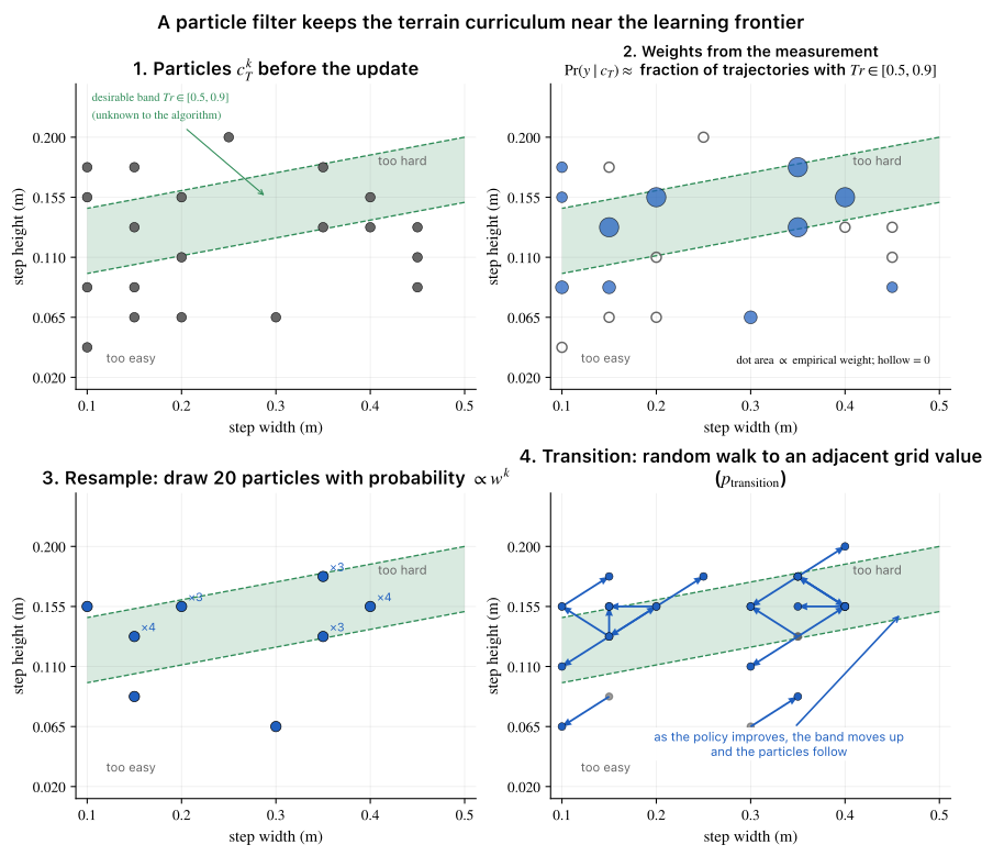
A synthetic cycle on the Stairs parameter plane (Table S2 ranges), in Algorithm S1's order: weight, resample, transition. Invented for illustration: the 20 particles (Table S3 uses 10 per terrain type), the grid spacing (the paper states none for ; Table S2's "grid size" is unexplained), the straight desirable band, and its upward drift in panel 4. S6 describes the Stairs distribution differently (below). The replay draw of line 20 is not drawn. In panel 2 dot area is the in-band fraction; hollow dots scored and cannot survive resampling.
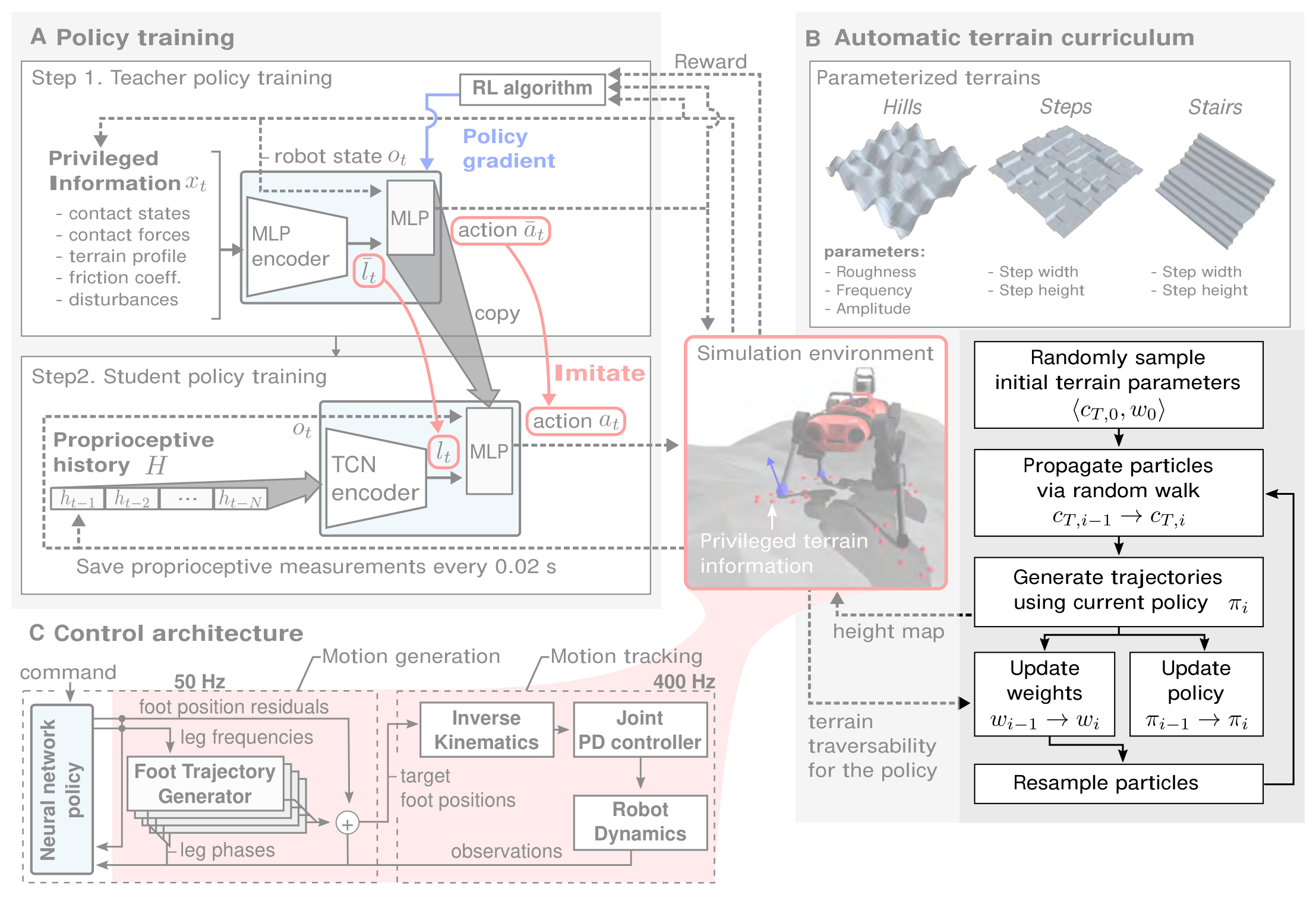
Fig. 4 (p. 7), the particle-filter loop of panel B highlighted. After an initial-sampling box, the paper's loop runs: propagate by random walk, generate trajectories with the current policy, update weights and policy from the same trajectories, resample. As a loop this is Algorithm S1's cycle entered at a different step; on the first pass the figure propagates before any rollout, while Algorithm S1 rolls out on the initial samples. The figure indexes particles, weights, and policy all with ; Algorithm S1 counts policy updates with and curriculum updates with , and weights are updated once per policy updates. The label does not mean the new weight is computed from the old one: line 16 has no previous-weight factor.
What separates Algorithm S1 from the SIR filter of the lectures:
- Target. A distribution of terrain parameters weighted by desirability for a policy that keeps changing, not a posterior over a hidden state.
- Transition. A designed random walk plus replay draws, not a known model of how anything evolves.
- Likelihood. Estimated from 60 trajectories pooled over a window in which the policy is updated ten times; it can be for every particle.
- Output. No estimate is formed; the particle set is used directly as the next training terrains.
- Bookkeeping. 10 particles per terrain type (Table S3); whether each type is weighted and resampled as its own filter is not stated.
S6, Fig. S1 · How the desirable set changes during training
The paper states the intent on p. 8: terrains are synthesised adaptively "according to the skill level of the trained policies at any given time". Fig. 4B's caption calls the maintained distribution "challenging but traversable by the policy" (p. 7). The evidence is S6 and Fig. S1 (pp. 16, 18), and only one of its panels shows change over training.
Fig. S1A–C is about Hills. Panel A shows example terrains with their parameters and traversability, as labelled in the figure:
| Fig. S1A panel | Roughness | Frequency | Amplitude | Traversability |
|---|---|---|---|---|
| i | 0.02 | 0.1 | 2.0 | 0.91 |
| ii | 0.15 | 0.3 | 2.0 | 0.56 |
| iii | 0.15 | 1.2 | 0.5 | 0.67 |
| iv | 0.15 | 1.2 | 2.0 | 0.15 |
Panels i and iv fall outside and ii and iii inside it, matching S6: undesirable terrains are either too easy or too difficult. Several labelled values lie outside the Table S2 ranges (roughness ; frequency and outside ); the paper does not explain this.
Panel B shows desirability estimated from 1000 trajectories of a fully trained teacher, with red crosses at the examples of A. Panel C shows the terrain profiles the particle filter sampled during the last 100 iterations of teacher training. S6 reads B and C together: the particle filter fits the latent distribution of desirable terrains, which has a bow shape in the frequency–amplitude marginal. B and C are end-of-training snapshots. They show that the particles match the desirable set at the end, not how that set moved.
Fig. S1D is about Stairs and is the one panel that shows the evolution of terrain parameters during training. S6 says the filter rejects short, steep steps (the upper-left area), initially focuses on wide, shallow steps (middle panels, particularly Iter. 50–60), and then broadens the distribution to include narrower steps (rightmost panels). S6 does not describe the initial spread, and neither S6 nor the caption says whether "Iter." counts policy updates or curriculum updates .
"The band moves" therefore means two things of different strength. By definition, changes whenever does, so the target of the filter changes during training. As evidence, the paper shows that change for one terrain type, Stairs, in S1D.
6 · Reading the evidence
🟡 · This chapter is short because the paper explains its own experiments well; what it assumes is the vocabulary.
Fig. 5 · Ablation logic, seeds, and intervals
An ablation removes one component while holding the rest fixed and measures what is lost. Fig. 5 does this three times: history length (B–D), privileged training versus direct RL (E–G), adaptive versus uniform terrains (H–J), each on three diagnostic tests, an omnidirectional slope, a discrete step, and a lateral push, with 100 trials per test.
Every model was trained five times with different random seeds and the error bars are 95 % confidence intervals. Two sources of randomness are folded into those bars: the trials, whose success rate is a binomial proportion with standard error at most , and the training runs themselves, whose outcome varies with initialisation and sampling. Five seeds is the field's convention and is small; the Roadmap's Section 5 (Paper Reading Roadmap) lists the paper that shows why single-seed results are not results. Read Fig. 5 by asking whether the intervals overlap, not by the height of the bars.
p.12 · The decoder probe: what the encoding contains, with an uncertainty
To see what the student's history encoding holds, the paper trains a decoder after the fact, with the policy frozen, from an intermediate layer of the TCN back to the privileged information . Discrete targets (contact states) use a cross-entropy loss. Continuous targets use a Gaussian negative log-likelihood in which the decoder predicts both a mean and a standard deviation per component (eq. 8):
This is heteroscedastic regression (Kendall and Gal 2017). The first term punishes an error more when the network claims to be certain; the second punishes claiming uncertainty. Per sample the loss is minimised at , so the predicted learns to track the actual error, and it can be read as the encoding's uncertainty. That is what Fig. 6B and Fig. S2 plot: the estimated elevation under the front feet rises when a foot hits a step, its uncertainty grows, and the uncertainty stays elevated afterwards on rough ground, which the paper reads as the encoding carrying terrain roughness.
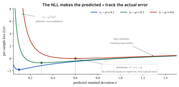
The two terms of the Gaussian negative log-likelihood pull in opposite directions and meet at .
One caution on reading a probe. That can be decoded from the features shows the information is present in them, not that the policy uses it. The saliency analysis is the paper's answer to the second question.
p.12 · Saliency
Eq. (9) defines the saliency of the -th past measurement as
the absolute sensitivity of the commanded foot height to each entry of the input window, summed over channels: one row of the input–output Jacobian in the sense of Matrix Calculus (Gradients) (Simonyan et al. 2013). Fig. 6C–D shows the saliency peaking at the moment the front foot hit the step and staying high through the following swing: the policy keeps attending to that one collision sample while it lifts the foot higher. Decoding showed the information was there; saliency shows it was used.
p.5 · Cost of transport
The paper's efficiency measure is the mechanical cost of transport,
positive mechanical power only (negative work, when an actuator brakes, is excluded), divided by weight times speed. It is dimensionless, so it compares machines and animals of different size; the reference is Collins et al. 2005 on passive-dynamic walkers.
Appendix A · Deep-learning vocabulary in Tables S5–S9
🟡 · A lookup table for reading the supplement's architecture and training tables, in the meaning each term has in this paper.
| Term | Meaning here | Where |
|---|---|---|
| MLP | fully connected layers with a nonlinearity after each; the teacher's encoder and both heads | Table S5 |
| , | a layer with units and that activation; ReLU follows every convolution, tanh the dense layers | Table S5 |
| id | identity map: the input passes to the next layer unchanged (the path of the teacher) | Table S5 |
| concatenate | join two vectors end to end into one input for the next layer | Table S5 |
| output layer | the 16 action components (policy), or the 64 latent components (encoder), or (decoder) | Table S5 |
| # param. | total trainable weights and biases; equalised across TCN variants for the ablation | Table S6 |
| 1-D conv, dilation, stride, filter size | see The DSP view: a causal 1-D convolution is an FIR filter with learned taps | Table S5 |
| receptive field | span of input samples one output depends on; TCN- | §4 |
| GRU | gated recurrent unit; a recurrent layer with a learned state | Table S5, S8 |
| truncated BPTT | backpropagation through time cut off after a fixed number of past steps | S8, Table S6 |
| batch size | samples per policy update (teacher, transitions) or per supervised update (student, ) | Tables S7, S8 |
| minibatch, epoch | one update uses a minibatch; one epoch passes once over the whole batch | Tables S8, S9 |
| Adam | adaptive-step-size variant of stochastic gradient descent | Tables S8, S9 |
| learning rate decay | : multiply by every updates | Tables S8, S9 |
| weight decay | an penalty on the weights added to the loss | Table S9 |
| encoder, latent, embedding | the compressing sub-network and its output vector | Table S5 |
| decoder, probe | a network trained from features back to a known quantity, policy frozen | p. 12, Table S9 |
| cross-entropy | the loss for classification targets (contact states) | p. 12 |
| negative log-likelihood | the loss for regression with a predicted uncertainty | eq. 8 |
| saliency | gradient of an output with respect to the inputs | eq. 9 |
| SGD time | wall-clock time of one gradient update | Table S6 |
Appendix B · Notation cheat sheet (S1)
| Symbol | Reading |
|---|---|
| , , | inertial frame, base frame, horizontal frame of leg |
| , | an axis of a frame: the -axis of , the -axis of the base |
| linear velocity of frame relative to frame , expressed in frame (frame on top, pair below, both on the left); so is the base velocity in base coordinates | |
| , | horizontal components, vertical component |
| unit vector; is the commanded direction | |
| target quantity | |
| the teacher's quantity | |
| horizontal base velocity projected on the commanded direction | |
| magnitude of the base velocity orthogonal to the commanded direction | |
| , , , | angular velocity, joint torque, joint angle, yaw |
| , | leg phase, leg frequency offset |
| , | foot position, foot position residual (in ) |
| gravity direction | |
| gap function of the -th possible contact pair; in contact | |
| , , , | index sets: all contacts, body contacts, foot contacts, swing legs |
| , | cardinality of a set or norm; norm |
| terrain parameter vector and its (bounded, discretised) space | |
| , | traversability, desirability (not a trace) |
| , , , | robot-measurable observation, privileged information, per-step student input, the window |
| , , , | teacher latent, student latent, teacher action, student action |
Study checklist
Close the note and answer these in your own words. Reopen only the section linked after the question.
- Why does the network output a modulation of a periodic motion instead of joint targets, and what does the trajectory generator supply that the residuals do not? → p.8 · Why the network does not output joint targets
- Why is the phase fed to the network as , and what is different about this phase compared with the one in your MPC? → p.8 · The phase variable, and why it is fed back as cosine and sine
- What would go wrong if foot targets were expressed in the base frame instead of ? → p.8 · The horizontal frame
- Give the two reasons the paper ends in joint position targets computed by analytic inverse kinematics. → p.8 · Analytic inverse kinematics
- In what sense is exploration noise "a standard deviation," and why can it be shaped per direction here? → Gaussian policies: exploration is a standard deviation
- Why is a fixed learning rate in parameter space the wrong knob, and what quantity replaces it? → Why a step size in parameter space is the wrong knob
- State the TRPO surrogate and constraint, and name the two substitutions that separate the algorithm from its theorem. → The TRPO problem and its guarantee
- Why is the Fisher matrix never formed, and what do the CG rows of Table S7 control? → From the constrained problem to the update rule
- Why does direct RL of the proprioceptive network fail while imitation of a privileged teacher succeeds? → p.3, p.6 · The problem: one scalar per step cannot teach two things
- What is covariate shift in imitation, why does it compound, and what does DAgger change? → p.9 · DAgger: label where the student goes
- Why must the expert be queryable at arbitrary states for DAgger, and why is that easy here? → p.9 · DAgger: label where the student goes
- Explain causal, dilated, and strided convolution in filter language, and compute a receptive field. → The DSP view: a causal 1-D convolution is an FIR filter with learned taps
- What was held fixed across TCN-1, TCN-20, and TCN-100, and why does it matter for the ablation? → Table S5 · TCN-N, and what the ablation held fixed
- Define traversability and desirability, say which of them is thresholded per trajectory and over how many trajectories the measurement probability is pooled, and give the paper's reason for not using the reward. → p.9 · Traversability and desirability: hard but passable as probabilities
- Map the pieces of the curriculum onto a textbook particle filter: what is tracked, what the measurement and likelihood are, and which pieces the paper states versus which are interpretation. → p.9 · What is filtered: the textbook particle filter, piece by piece
- Walk through Algorithm S1: why does the weight line carry no previous-weight factor, why are the replay draw and the random walk the only ways a value outside the current set can enter, which of the two can produce a value never visited before, and what does the paper say the replay memory is for? → Algorithm S1 · One iteration of sequential importance resampling
- What does a decoder probe show, and what does it not show? → p.12 · The decoder probe: what the encoding contains, with an uncertainty
Gaps to close on your own
- TRPO in full. Schulman et al. 2015, Trust Region Policy Optimization, §3–§6: the proof of the improvement bound, the max-to-mean KL heuristic, and the Fisher-vector product trick. The conjugate gradient method itself is a numerical linear algebra topic: solve for symmetric positive definite using only products (a candidate for Linear Algebra Essentials when it blocks again).
- PPO. The successor that replaced the constraint by a clipped ratio; already in Zotero and next on the Paper Reading Roadmap. Read Engstrom et al. 2020 alongside it.
- DAgger's guarantee. Ross, Gordon, and Bagnell 2011, Section 3 (Theorems 3.1–3.2), and the role of the mixing schedule . The paper does not say whether it mixed teacher and student control in early iterations or ran the student alone from the start.
- Learning by cheating. Chen, Zhou, Koltun, and Krähenbühl, CoRL 2019: the source of the two-stage pattern, in driving.
- TCN. Bai, Kolter, and Koltun 2018, §3: residual blocks and weight normalisation are part of their TCN; Table S5 does not say whether either was used here.
- Particle filters in general. Bayes and Particle Filters teaches the path from the Bayes filter to SIR, and Particle Filter is the one-page version. The series assumes a likelihood evaluated exactly and a target fixed by known transition and measurement models. Three things in §5 have no lecture behind them: a likelihood estimated from trajectories (random weights, and likelihood estimates that can all be , leaving the normalising denominator at ), a measurement model that changes with a policy trained on the particles' own rollouts, and a replay memory under which the next particle set can depend on more than the current set, so the process is Markov if the memory is counted as part of the state. 🟡 until a state-estimation paper makes it 🔴.
- PMTG and the horizontal frame. Iscen et al. 2018 (PMTG) and Barasuol et al. 2013 (horizontal frames, reactive controller framework). Both are short.
- Analytic IK for the actual ANYmal leg. The textbook two-link version above ignores the fixed offsets between the HAA, HFE, and KFE axes. The lab's open-source kinematics is the reference if it ever needs implementing.
- ⚡ Where the origin of sits. p. 8 places the horizontal frame below the hip at the nominal reach of the leg, and eq. (11) puts the stance foot below that origin along . Taken literally that is half a metre under the default foothold. The self-consistent reading is that the in eq. (11) is the nominal reach, measured from the hip — eq. (11) written in a hip-anchored frame carrying 's orientation, its stance value landing on the origin of . Do not stack the two distances. The paper also does not say which direction "below the hip" is measured along, and Barasuol et al. 2013 is the reference for the construction.
- ⚡ 50 Hz or 400 Hz. Fig. 4C labels motion generation and motion tracking , and the history is saved every ; S2 says "the neural network policy runs at 400 Hz on an onboard CPU." Both are in the paper. The consistent reading is that the tracking loop, not the network's input rate, runs at , but the paper does not resolve it.
- Not stated by the paper. Whether the teacher's advantage used a learned value baseline or generalised advantage estimation; the per-coordinate values; how the student's rollouts were mixed with the teacher's, if at all.
Language notes
Phrasings from the paper worth keeping for your own writing.
| Expression | Use |
|---|---|
| feel out the environment with its body | describing a blind controller that probes by contact |
| off-the-shelf | a standard component used without modification |
| maximize the didactic benefit of each episode | justifying a curriculum: every sample should teach |
| neither too challenging nor trivial | the sweet spot a curriculum targets |
| distilled into a proprioceptive student policy | compressing a large or privileged model into a deployable one |
| within reasonable time budgets | conceding a method fails for cost reasons, not in principle |
| affords transparent control over the input history length | naming a design advantage of an architecture |
| is known to be robust to hyperparameter settings | citing prior evidence for a choice |
| a strong indicator that | drawing a conclusion from indirect evidence, carefully |
| precluding reliance on frameworks that may require seconds of computation per time step | ruling out an option by cost |
| expedite the deployment of | stating an engineering impact |
| the feasible range of target speeds is often unclear | motivating a direction-only command |
| purely from proprioceptive observations | stating what an inference does not use |
| elicit (multiple gaits) | future work: bringing out a behaviour by changing the training protocol |
| manifest higher foot clearance | describing an emergent behaviour without claiming a mechanism |
Related: Lee 2020 - Learning Quadrupedal Locomotion over Challenging Terrain · Hwangbo 2019 - Learning Agile Motor Skills (ANYmal) · Lecture 7 · Policy Gradient · Position Actions as Impedance Control in Robot RL · Bounded Kernel Rewards in Robot RL · Sensors vs Simulator in Robot RL · Importance Sampling in Off-Policy RL · Markov Decision Process (MDP) · Convex MPC Biped (My Article) · Matrix Calculus (Gradients) · Paper Reading Roadmap · Academic Baseline