Lecture 5 · Model-Free Control

Slides: David Silver - RL Course (UCL 2015) · Previous: Lecture 4 · Model-Free Prediction · Next: Lecture 6 · Value Function Approximation

Read this instead of watching. Each slide is embedded below with only what the slide itself does not say — the reasoning, the caveats, and the questions worth being able to answer.

The one idea

Lecture 4 answered "given $\pi$ , how do I estimate $v_\pi$ ?" Lecture 5 drops that estimator into the generalized policy iteration (GPI) loop to find $q_*$ . Everything else is a variation on which estimator goes in which slot.

	Policy evaluation ↑	Policy improvement ↓	Algorithm
Dynamic programming (L3)	iterative policy evaluation	greedy	policy iteration
Monte-Carlo	MC evaluation of $Q$	$\epsilon$ -greedy	GLIE MC control
Temporal-difference	Sarsa	$\epsilon$ -greedy	Sarsa, Sarsa( $\lambda$ )
TD, off-policy	Q-learning	greedy target, $\epsilon$ -greedy behavior	Q-learning

Two substitutions make the whole lecture work.

Substitution 1 — use

Q

, not

V

Greedy improvement on $V$ needs one-step lookahead, $\pi'(s)=\arg\max_a\big(\mathcal{R}^a_s+\gamma\mathcal{P}^a_{ss'}V(s')\big)$ , and that lookahead is a model. With $Q$ it collapses to $\pi'(s)=\arg\max_a Q(s,a)$ — no model at all.
$Q$ is a cache of the lookahead. Storing values per action is what buys model-freedom.

Substitution 2 — use

\epsilon

-greedy, not greedy

DP swept every state. Here you only see what you visit, so a greedy policy can lock onto a wrong belief it will never revisit. Perpetual exploration is not a refinement — it is a correctness requirement.

1 · Why model-free control
2 · Making GPI model-free
3 · Exploration and ε-greedy
4 · GLIE Monte-Carlo control
5 · Sarsa
6 · Sarsa(λ)
7 · Off-policy learning
8 · Q-learning
9 · The DP–TD correspondence
Study checklist
Gaps to close on your own
Language notes

1 · Why model-free control

p.4 · Uses of Model-Free Control ⏱ 2:17

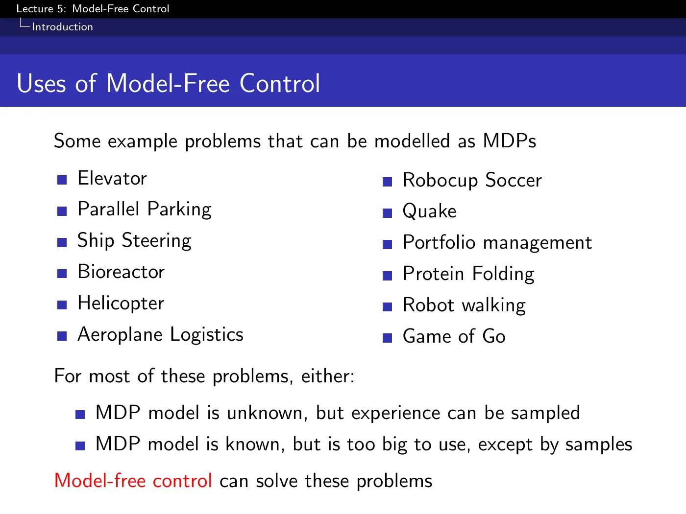
Model-free applies in two situations, and the second is the one people forget:

The MDP model is unknown.
The model is known but too large to use, except by sampling.

Real-world physics is case 2. You could in principle write down the dynamics, but no one wants to integrate over every atom — you sample instead. So model-free is not only a response to ignorance; it is a response to lookahead being more expensive than experience. → Model-Free vs Model-Based RL

p.5 · On- and Off-Policy Learning ⏱ 3:47

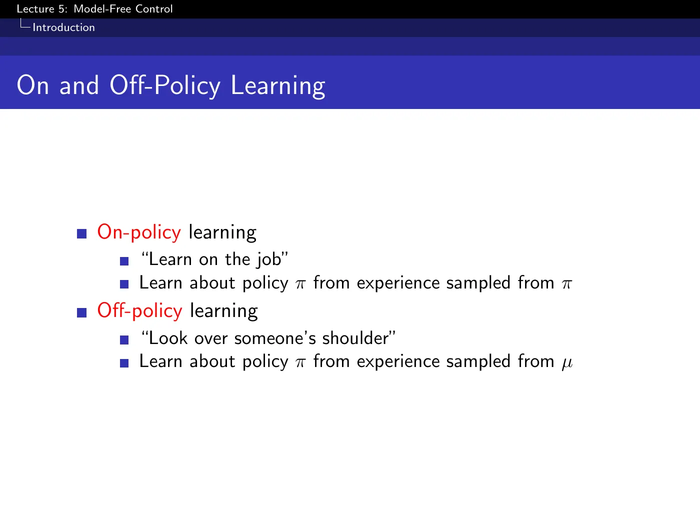
On-policy — learn on the job. Sample from $\pi$ , evaluate $\pi$ .
Off-policy — look over someone's shoulder. Sample from $\mu$ , evaluate $\pi$ .

The off-policy goal is stronger than imitation. Watching a human teleoperate an arm, you do not want to copy the trajectory — you want to conclude "you could have collected more reward by going this other way."

2 · Making GPI model-free

p.6–7 · Generalized Policy Iteration ⏱ 5:18

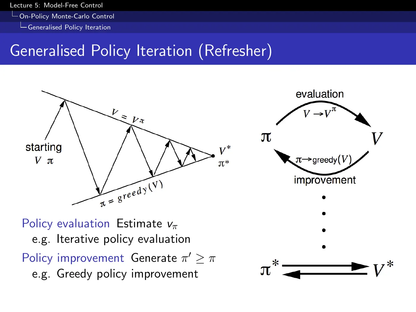
Up = evaluate, down = act greedily. Convergence of this cycle was settled in L3 → Contraction Mapping & Bellman Convergence. The only question now is what goes in each slot.

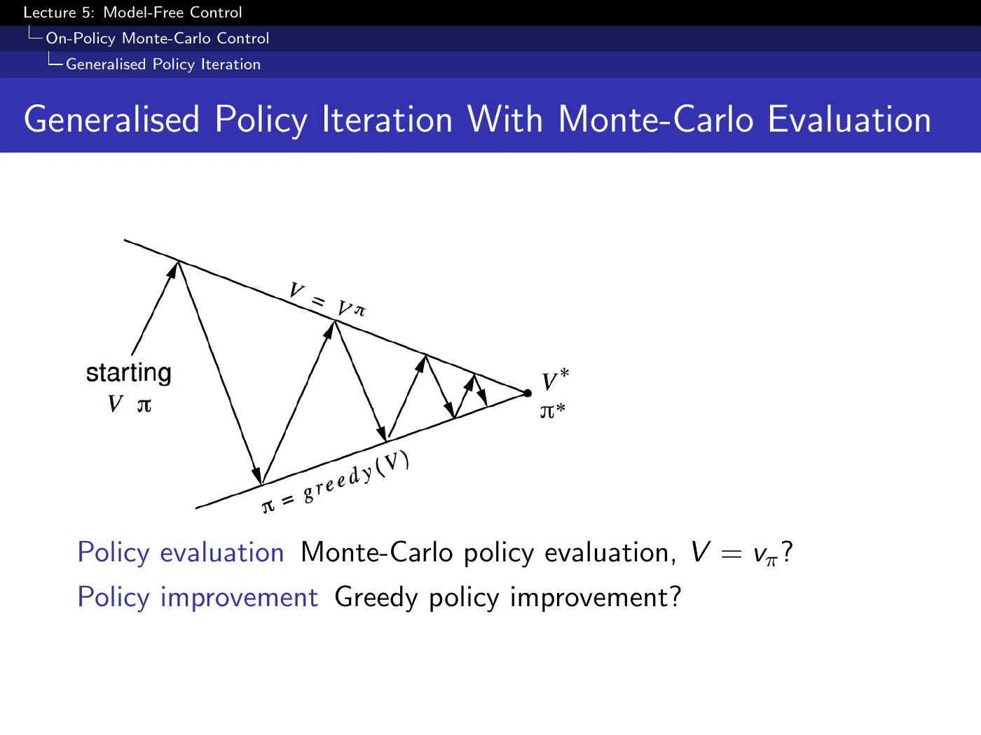
Plug MC evaluation straight into GPI. What breaks?

Three things, in order of depth.

Improvement is not model-free. Acting greedily w.r.t. $V$ needs the transition model. → fixed on p.8 by switching to $Q$ .
Exploration is not guaranteed. A greedy policy may never visit large parts of the state space, so those values stay wrong forever. → fixed on p.11 by $\epsilon$ -greedy.
It is slow. Full MC evaluation costs many episodes per improvement step. → fixed on p.14 (improve every episode) and p.19 (switch to TD).

p.8–9 · Model-Free Policy Iteration Using Q ⏱ 9:54

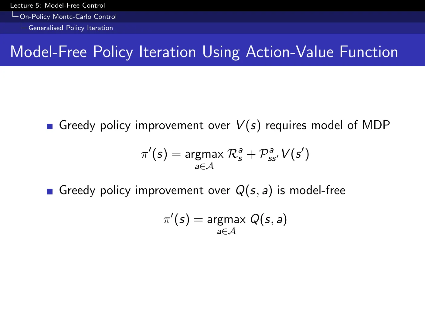
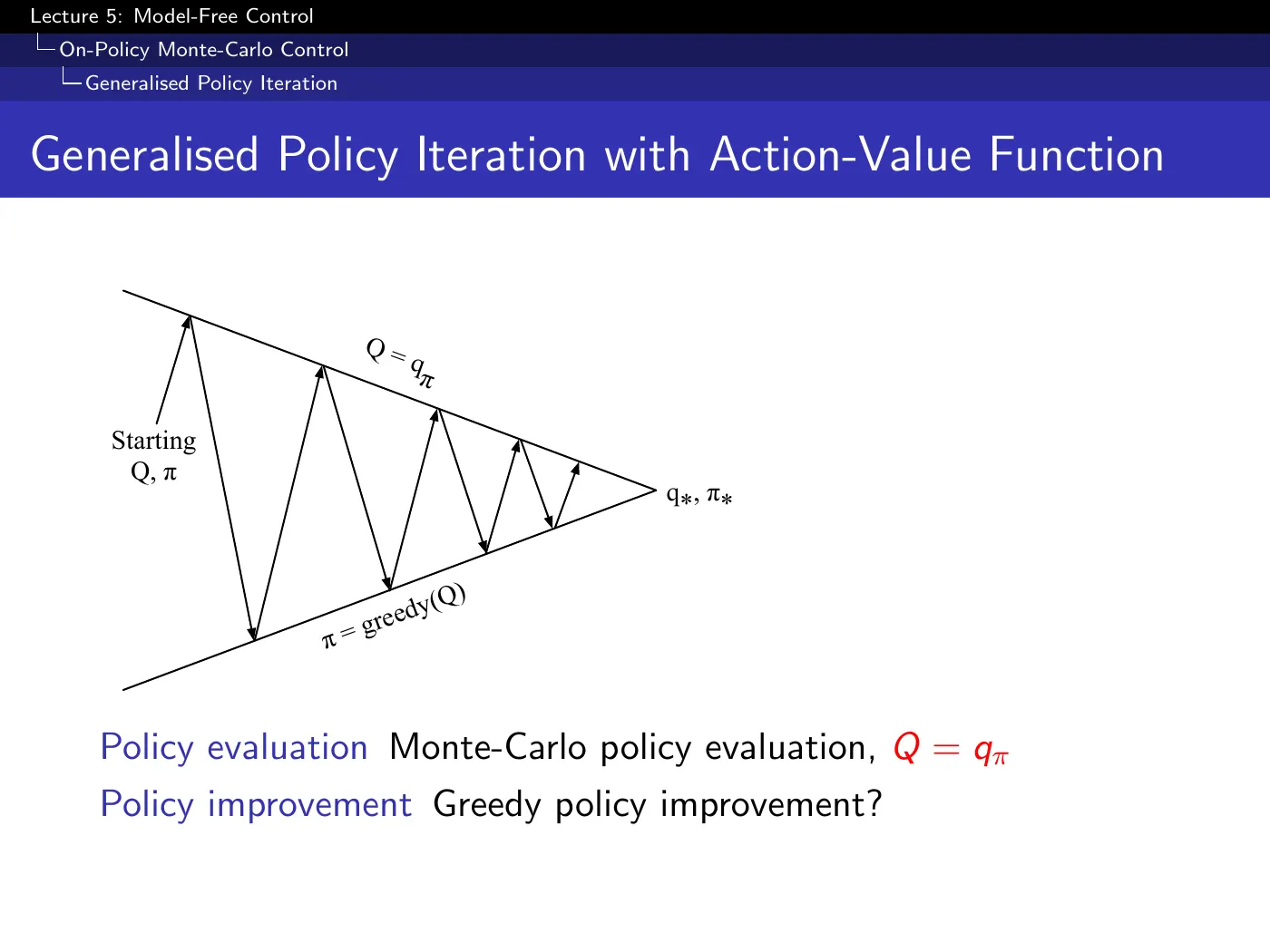
\underbrace{\pi'(s)=\arg\max_{a\in\mathcal{A}}\Big(\mathcal{R}^a_s+\gamma\textstyle\sum_{s'}\mathcal{P}^a_{ss'}V(s')\Big)}_{\text{needs a model}} \qquad \underbrace{\pi'(s)=\arg\max_{a\in\mathcal{A}}Q(s,a)}_{\text{model-free}}

Problem 1 is now gone. Problem 2 is still open — the down-arrow is still fully greedy.

3 · Exploration and ε-greedy

p.10 · Example of Greedy Action Selection ⏱ 12:56

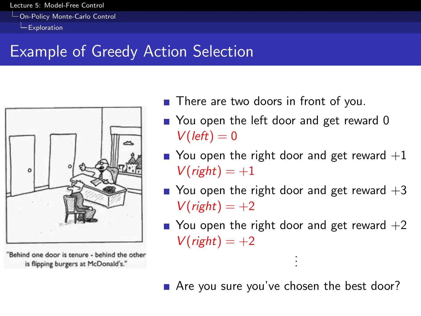
A two-armed bandit. Open the left door once, see $0$ , and greedy behavior never opens it again — even though a single sample says almost nothing about its true value.

The failure is not "greedy is suboptimal." It is that you get trapped inside a belief you have no mechanism to correct. Full treatment in L9.

p.11 · ε-Greedy Exploration ⏱ 15:13

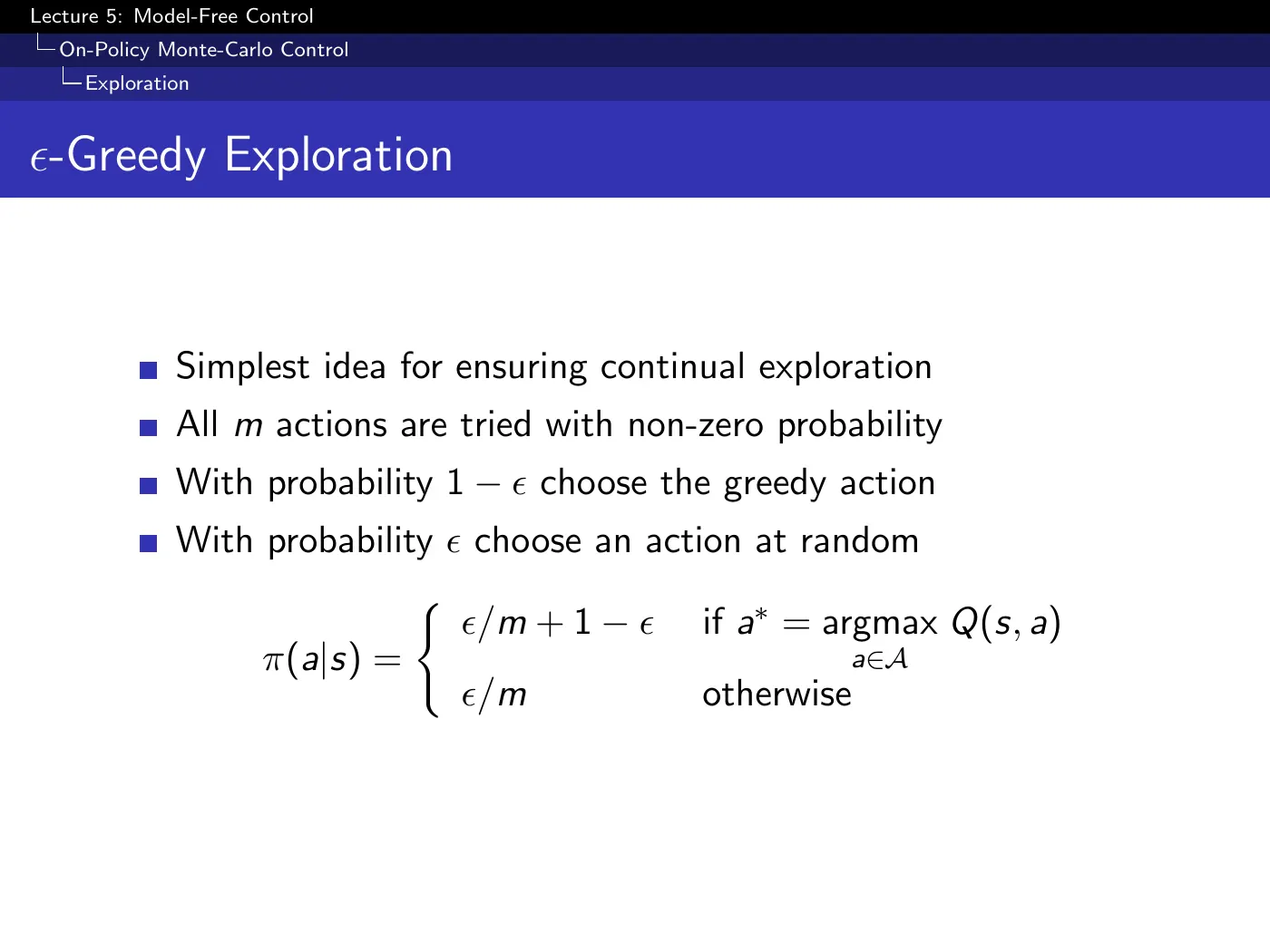
\pi(a|s)=\begin{cases} \epsilon/m+1-\epsilon & \text{if } a^*=\arg\max_{a\in\mathcal{A}}Q(s,a)\\[4pt] \epsilon/m & \text{otherwise} \end{cases}

Flip a coin: explore uniformly with probability $\epsilon$ , act greedily otherwise. The extra $\epsilon/m$ on the greedy action accounts for picking it by chance during exploration.

Naive as it looks, it is surprisingly hard to beat in practice.

p.12 · ε-Greedy Policy Improvement ⏱ 17:31

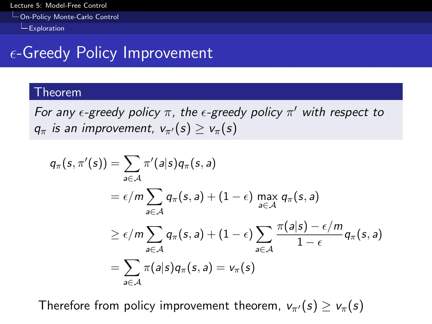
The whole proof rests on one inequality — a max dominates any convex combination:

\max_{a}q_\pi(s,a)\;\ge\;\sum_{a}w_a\,q_\pi(s,a),\qquad w_a\ge 0,\ \textstyle\sum_a w_a=1

The trick is the choice of weights. Take

w_a=\frac{\pi(a|s)-\epsilon/m}{1-\epsilon}

and the $1-\epsilon$ factors cancel, the terms collapse, and what remains is exactly $\sum_a \pi(a|s)q_\pi(s,a)=v_\pi(s)$ . Hence $q_\pi(s,\pi'(s))\ge v_\pi(s)$ .

That is a one-step result. Extending it to $v_{\pi'}\ge v_\pi$ reuses the telescoping argument from the L3 policy improvement theorem — not re-derived here.

What this theorem does not give you

It says nothing about how much to explore or how fast $\epsilon$ should decay. Monotone improvement holds for any fixed $\epsilon$ . Choosing a schedule is a separate problem, answered by GLIE.

4 · GLIE Monte-Carlo control

p.13–14 · Monte-Carlo Policy Iteration → Control ⏱ 22:04

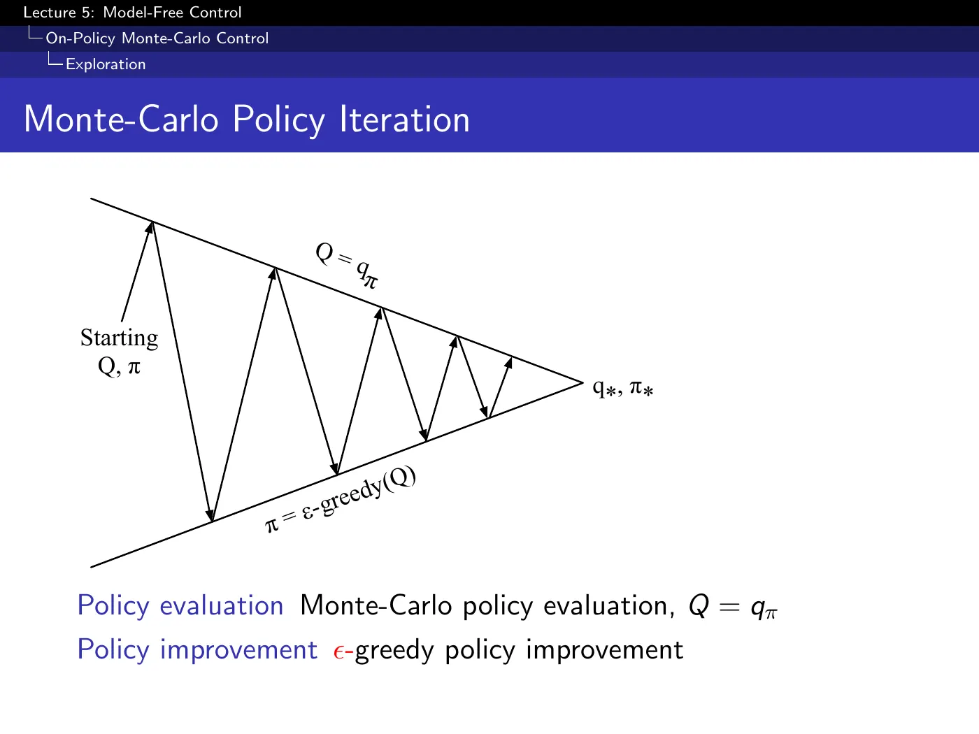
Both slots are now replaced: evaluation = MC on $Q$ , improvement = $\epsilon$ -greedy. The down-arrow no longer reaches a deterministic policy, and that residual stochasticity is what keeps exploration alive.

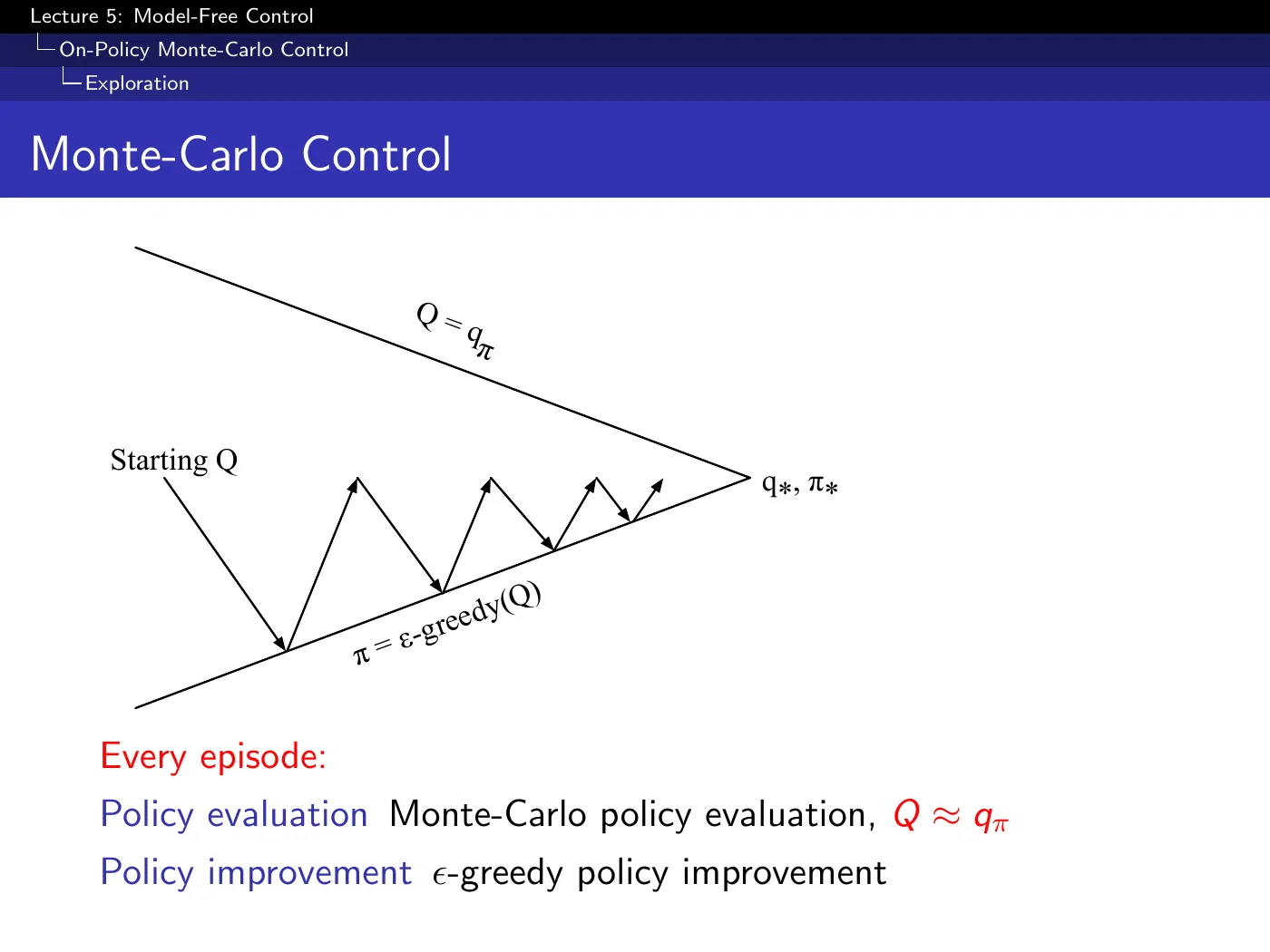
There is no reason to evaluate a policy to convergence before improving it — the same argument as in DP. Push it to the limit: improve after every single episode.

The principle that runs through the rest of the lecture

Always act greedily with respect to the freshest estimate you have. Waiting to collect more data before improving means generating that data with a policy you already know is stale. This is why the loop tightens from batch of episodes → one episode → one time-step.

p.15 · GLIE ⏱ 25:15

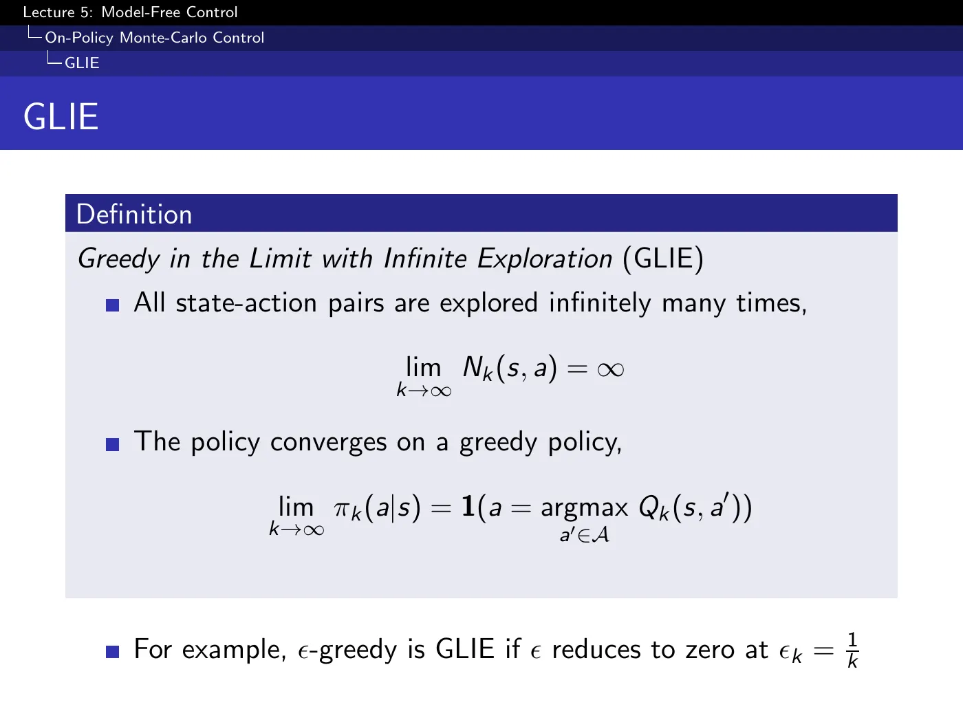
Greedy in the Limit with Infinite Exploration — two conditions, each doing distinct work:

Condition	Why it is needed
$\lim_{k\to\infty}N_k(s,a)=\infty$	Unvisited pairs keep wrong estimates forever
$\lim_{k\to\infty}\pi_k(a\mid s)=\mathbf{1}\!\left(a=\arg\max_{a'}Q_k(s,a')\right)$	The Bellman optimality equation contains a $\max$ . A policy that stays soft satisfies the expectation equation for that soft policy — you converge to some $q_\pi$ , not to $q_*$

$\epsilon_k=1/k$ satisfies both. It is a valid schedule, not a good one.

p.16 · GLIE Monte-Carlo Control ⏱ 28:17

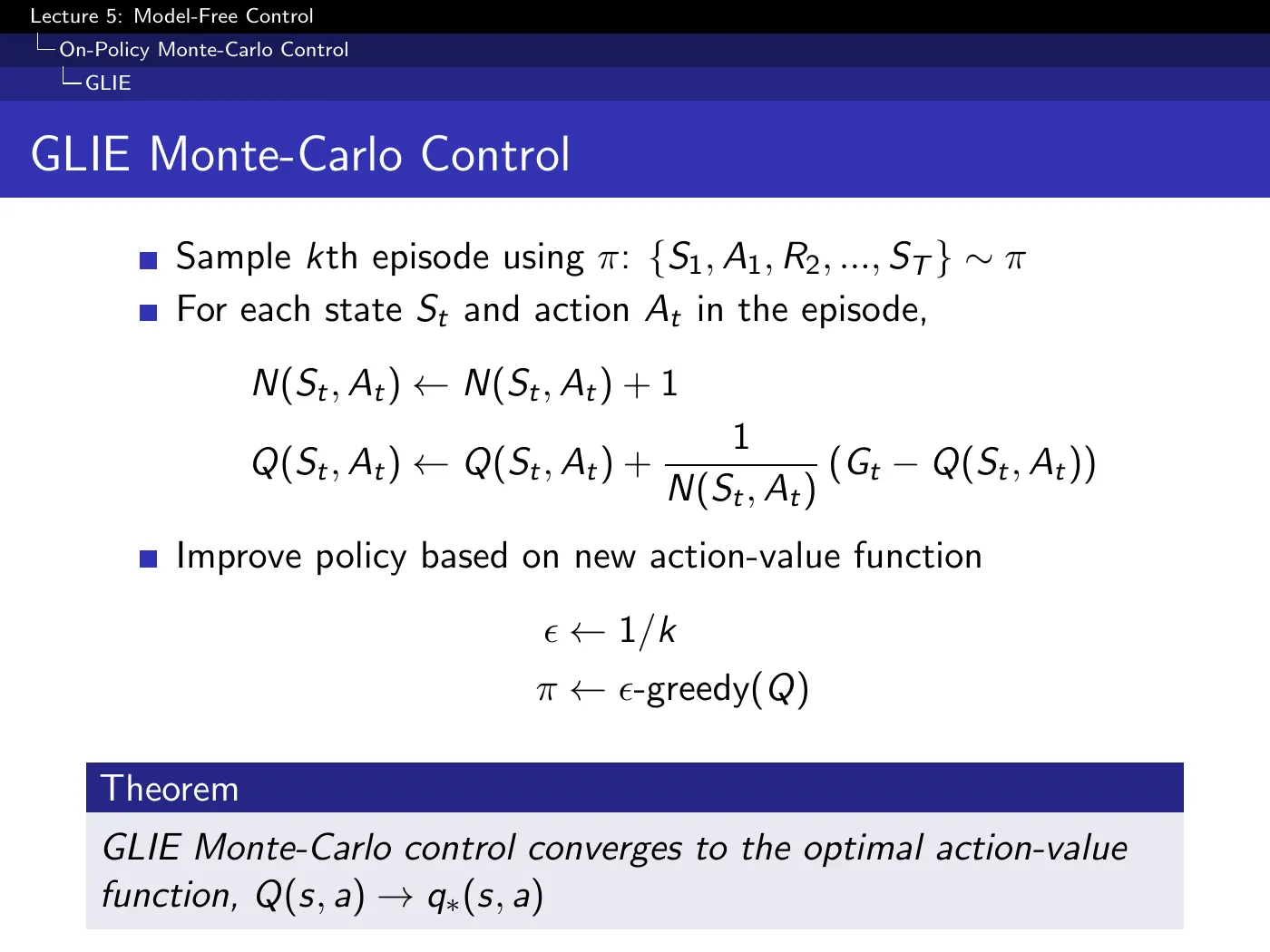
N(S_t,A_t)\leftarrow N(S_t,A_t)+1,\qquad Q(S_t,A_t)\leftarrow Q(S_t,A_t)+\frac{1}{N(S_t,A_t)}\big(G_t-Q(S_t,A_t)\big)

This is not an i.i.d. mean

The returns being averaged come from a sequence of different policies, since $\pi$ improves as you go. It is only GLIE that rescues this: as $\pi_k$ approaches greedy, the early samples from bad policies are progressively dominated, and the average converges on the quantity you actually care about.

Does the initialization of

Q

matter?

With a $1/N$ step size, not at all. On the first visit to a pair, $N=1$ , so the update is $Q\leftarrow Q+1\cdot(G_t-Q)=G_t$ — the initial value is overwritten exactly, in theory and in practice.
With a constant $\alpha$ it matters a great deal, because every update only moves a fraction of the way from wherever you started. That applies to Sarsa and Q-learning below, not to this algorithm.

Implementation note. Do not store $\pi$ . Keep $Q$ , and when it is time to act, flip a coin against the current $\epsilon_k$ . The policy is implicit in $Q$ plus the schedule.

p.17–18 · Blackjack ⏱ 34:39

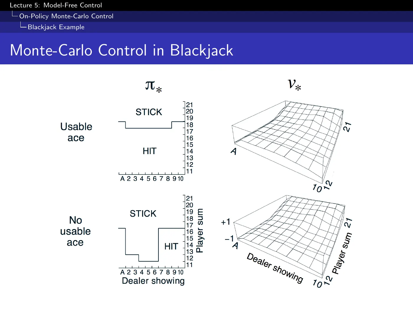
L4 asked "how much do I lose with this fixed policy?" (prediction). Same problem, now control: "how should I actually play?" The plots show $v_*$ rather than $Q$ — the action dimension is collapsed for legibility; internally the algorithm holds $Q$ .

The learned policy is not a simple threshold on your own hand. It sticks on low totals precisely where the dealer's upcard makes the dealer likely to bust — optimal play sometimes means declining to act and letting the opponent lose. A usable ace shifts the whole boundary toward hitting, since counting it as 1 or 11 removes the downside.

5 · Sarsa

p.19 · MC vs. TD Control ⏱ 38:26

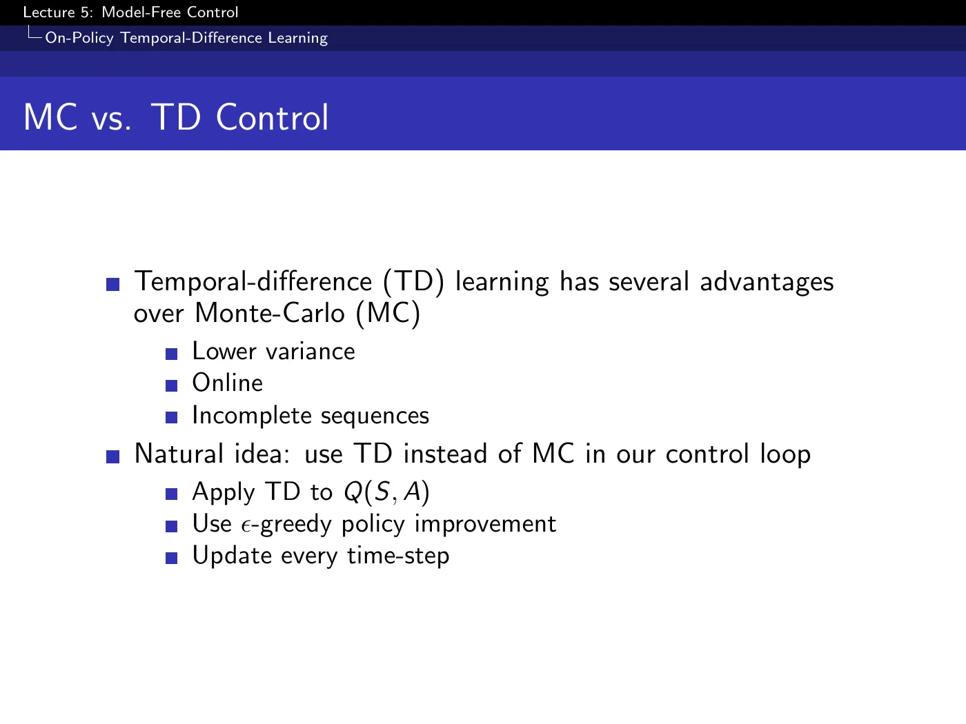
Lower variance, online, works on incomplete sequences — plus a fourth advantage the slide omits: TD is what makes off-policy learning viable at all (see p.33).

p.20–21 · The Sarsa Update ⏱ 39:57

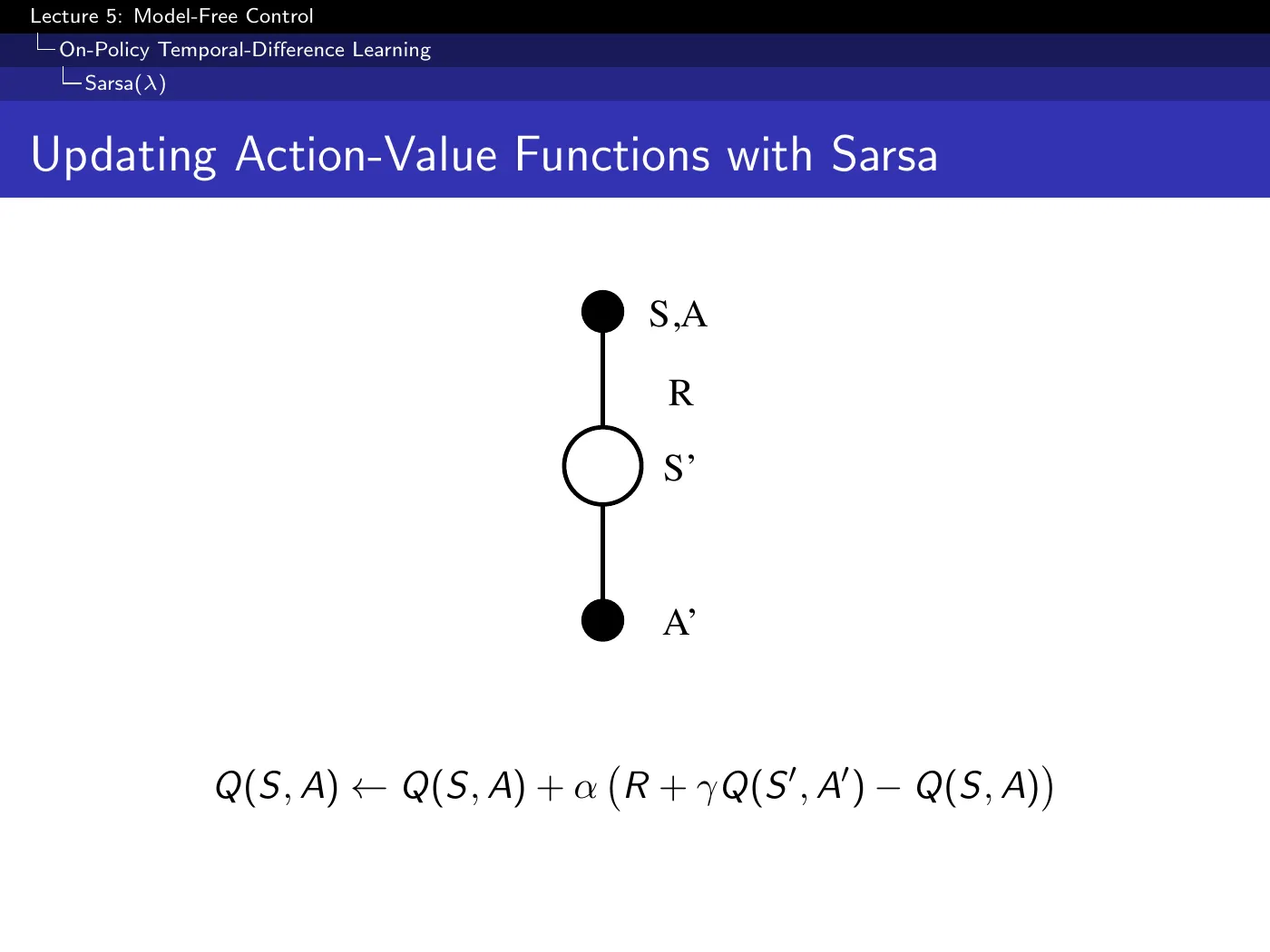
Q(S,A)\leftarrow Q(S,A)+\alpha\big(R+\gamma Q(S',A')-Q(S,A)\big)

The name is the update's data dependency, and it involves two different kinds of sampling:

Step	Sampled from
$S,A \rightarrow R,S'$	the environment
$S' \rightarrow A'$	your own policy

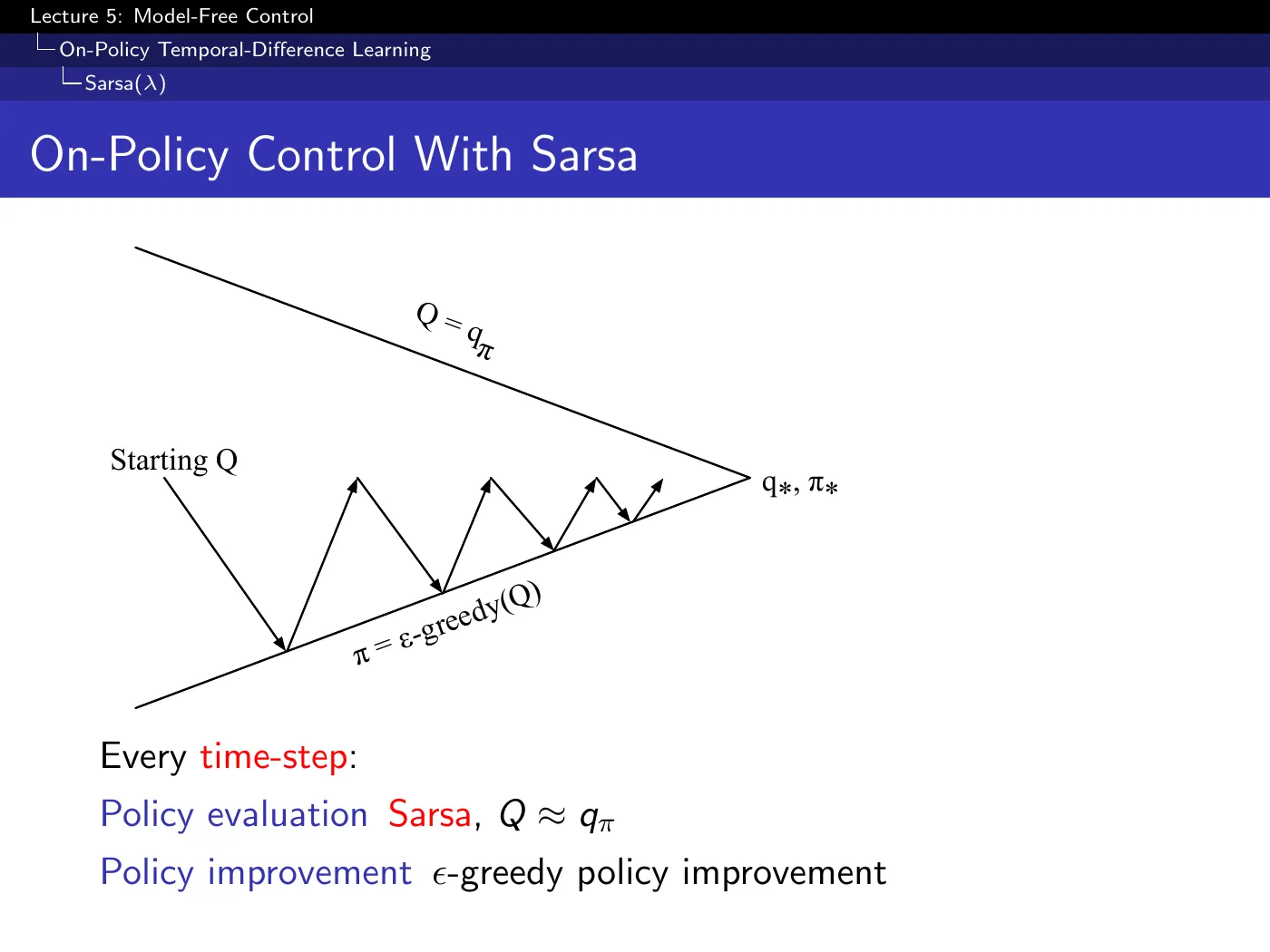
The GPI loop now runs at every time-step: update one cell of $Q$ , immediately improve. In a looping environment this means that when you return to a state you already behave differently.

p.22 · Sarsa Algorithm ⏱ 44:29

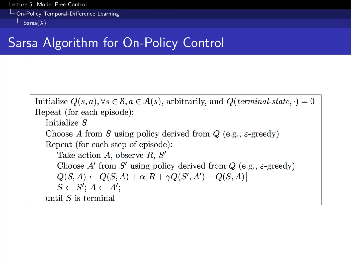
$Q$ is a lookup table, arbitrarily initialized (zeros are fine — but see the constant- $\alpha$ caveat above). The outer loop is over episodes; the loop that matters is over steps.

Where does

A'

come from, and why is it legitimate to bootstrap from an action you have not been rewarded for yet?

$S'$ comes from the environment; $A'$ you draw from your current policy, and you then carry it forward as the next step's $A$ — one policy sample per step.

The target $R+\gamma Q(S',A')$ is a sample of the Bellman expectation equation for $q_\pi$ , whose right-hand side splits in two:

$R$ and $S'$ — an expectation over the environment;
$Q(S',A')$ — an expectation over your own policy, from $S'$ onward.

That second term is precisely the thing being estimated. So the action must be drawn from the policy under evaluation for the target to be valid.

Sarsa is therefore on-policy by construction, not by convention. Breaking that constraint is exactly what Q-learning does, and it needs a different Bellman equation to stay valid.

p.23 · Convergence of Sarsa ⏱ 48:14

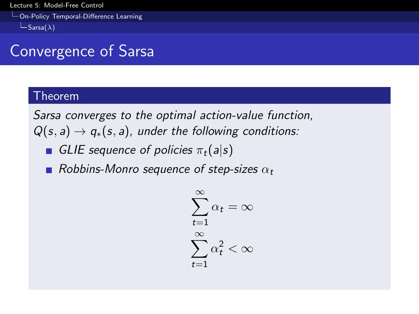
GLIE policies, plus Robbins-Monro step sizes:

\sum_{t=1}^{\infty}\alpha_t=\infty \quad\text{(you can travel arbitrarily far from a bad initial estimate)}

\sum_{t=1}^{\infty}\alpha_t^2<\infty \quad\text{(the updates must eventually vanish, or noise keeps rattling the policy)}

Theory vs. practice — stated outright in the lecture

In practice people commonly ignore both conditions, run a fixed $\alpha$ and a fixed $\epsilon$ , and Sarsa still works. That is an empirical observation, not a theorem — and the very next example does exactly this.

p.24–25 · Windy Gridworld ⏱ 49:46

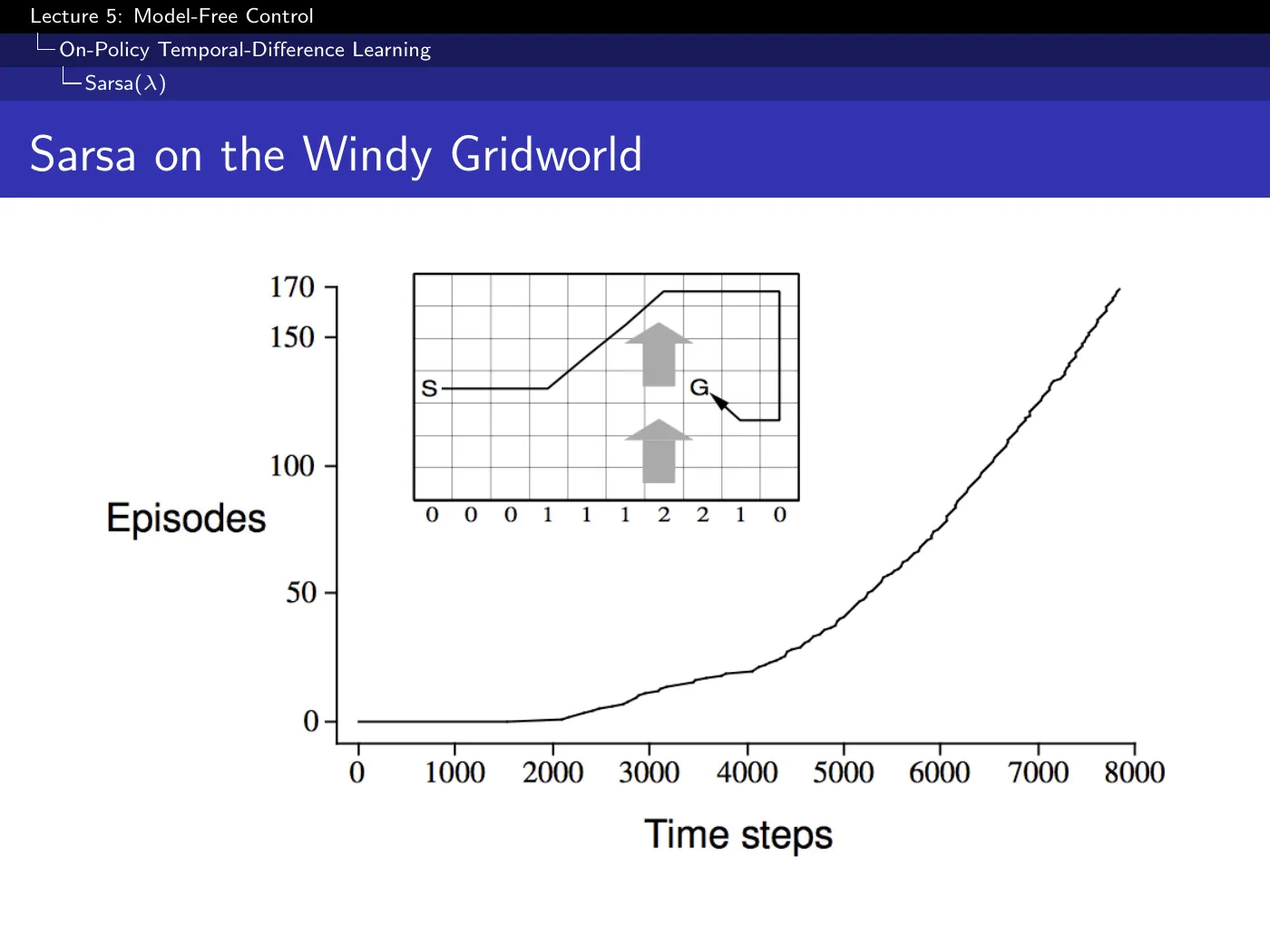
Read the axes carefully — this is the most misread plot in the lecture

The x-axis is time steps, not episodes. The y-axis is cumulative episodes completed. So the slope is $1/(\text{episode length})$ , and a steeper curve means shorter episodes.

The first episode takes about 2,000 steps — an undirected walk, biased upward by the wind, stumbling onto the goal by luck.
After the first success the curve bends sharply: once there is any signal, bootstrapping compounds it.
The final slope corresponds to a near-optimal path length. It never becomes perfectly straight because $\epsilon$ is not decayed, so exploratory actions keep being injected.

6 · Sarsa(λ)

p.26 · n-Step Sarsa ⏱ 53:40

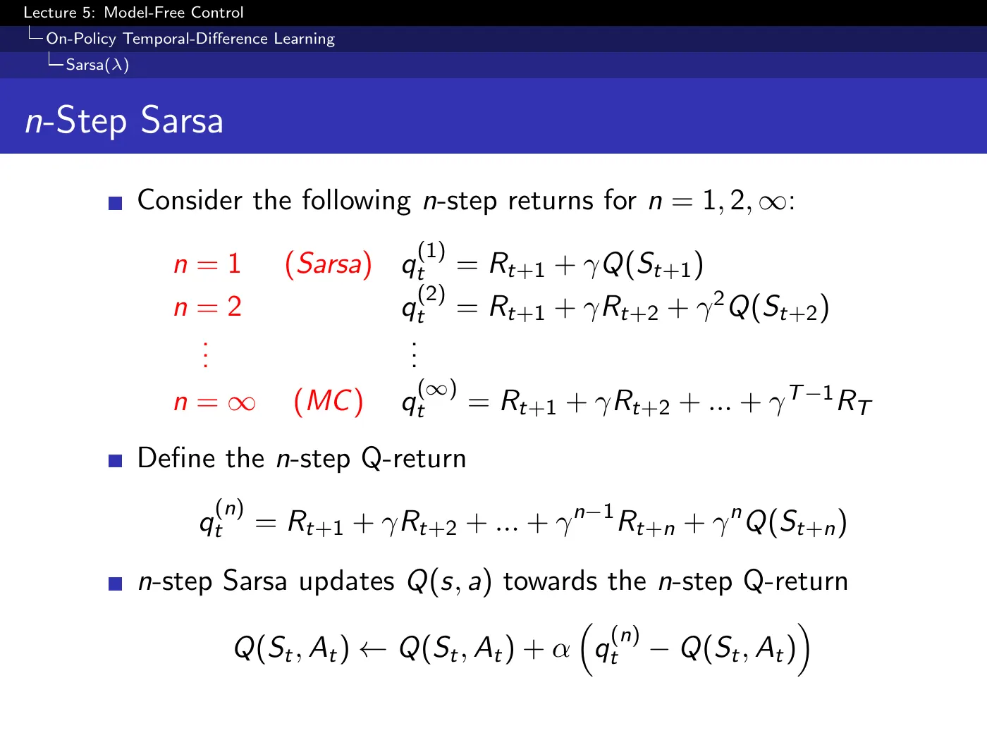
q_t^{(n)}=R_{t+1}+\gamma R_{t+2}+\dots+\gamma^{n-1}R_{t+n}+\gamma^{n}Q(S_{t+n}),\qquad Q(S_t,A_t)\leftarrow Q(S_t,A_t)+\alpha\big(q_t^{(n)}-Q(S_t,A_t)\big)

$n=1$ is Sarsa, $n=\infty$ is Monte-Carlo. Same spectrum as L4, now on $Q$ .

Changing $n$ changes how the target is built, never what is being estimated. The quantity is always the full return $q_\pi(s,a)=\mathbb{E}_\pi[G_t\mid S_t=s,A_t=a]$ ; an $n$ -step target simply measures the first $n$ rewards explicitly and compresses the infinite remainder into one $Q$ . Keep this straight — the same distinction returns in L6, where function approximation changes the representation of $Q$ without touching what $Q$ means.

p.27 · Forward View ⏱ 56:43

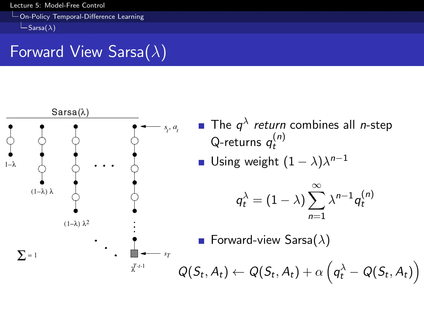
q_t^{\lambda}=(1-\lambda)\sum_{n=1}^{\infty}\lambda^{n-1}q_t^{(n)},\qquad Q(S_t,A_t)\leftarrow Q(S_t,A_t)+\alpha\big(q_t^{\lambda}-Q(S_t,A_t)\big)

$(1-\lambda)$ is only a normalizer making the geometric weights sum to 1 — do not read meaning into it. $\lambda=0$ recovers Sarsa, $\lambda=1$ recovers MC, and in between is a bias-variance dial.

The defect: $q_t^{\lambda}$ cannot be computed until the episode ends, so this is not online — and some problems have no episode boundary at all.

p.28–29 · Backward View ⏱ 1:00:30

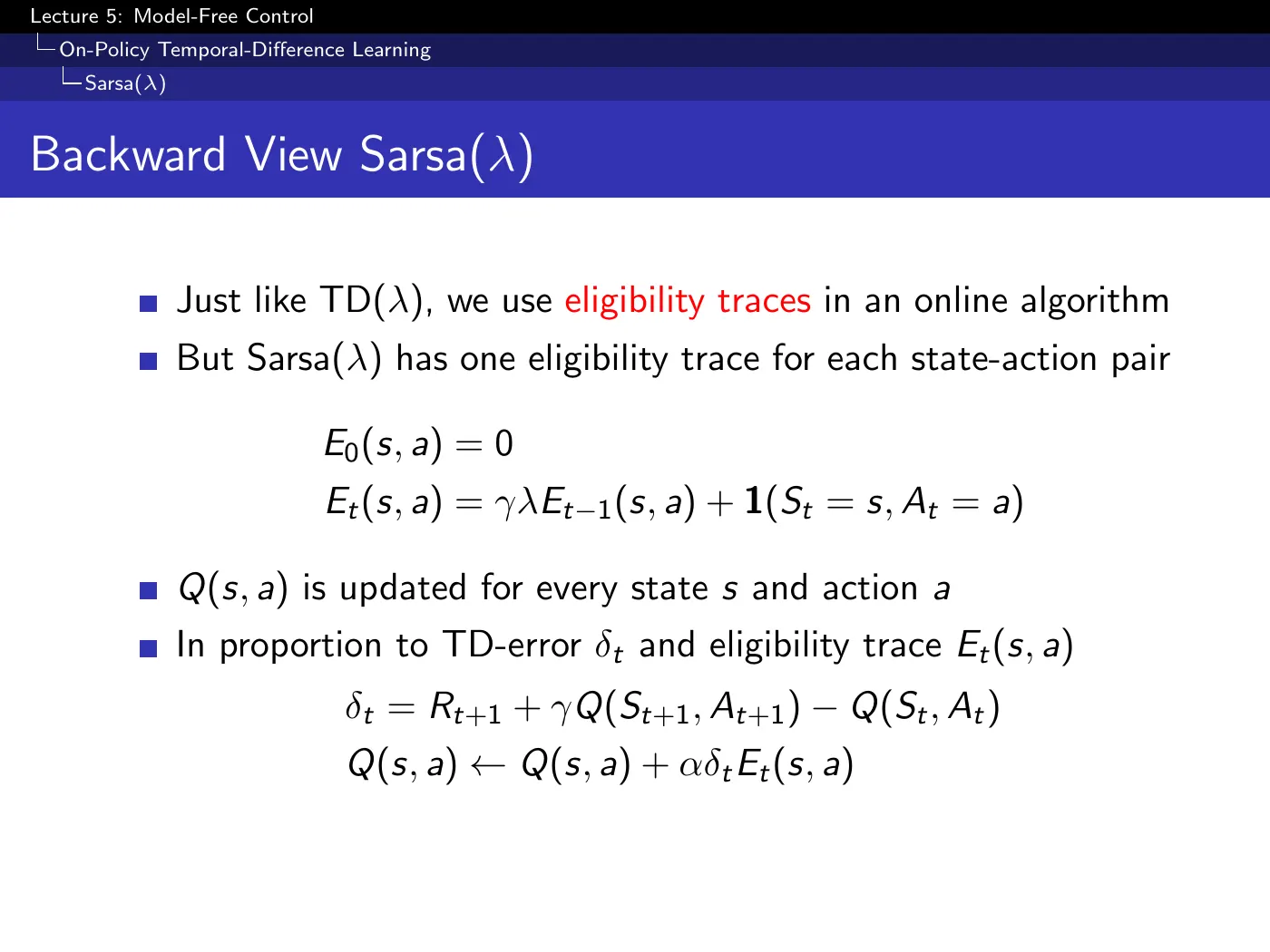
E_t(s,a)=\gamma\lambda E_{t-1}(s,a)+\mathbf{1}(S_t=s,A_t=a)

\delta_t=R_{t+1}+\gamma Q(S_{t+1},A_{t+1})-Q(S_t,A_t),\qquad Q(s,a)\leftarrow Q(s,a)+\alpha\,\delta_t\,E_t(s,a)\ \ \forall (s,a)

The eligibility trace is a credit assignment device: when a reward finally arrives, which state-action pairs deserve the blame or the credit? Two heuristics, combined — recency and frequency. Note the trace decays by $\gamma\lambda$ , not $\lambda$ alone.

The asymmetry that trips people up in implementation

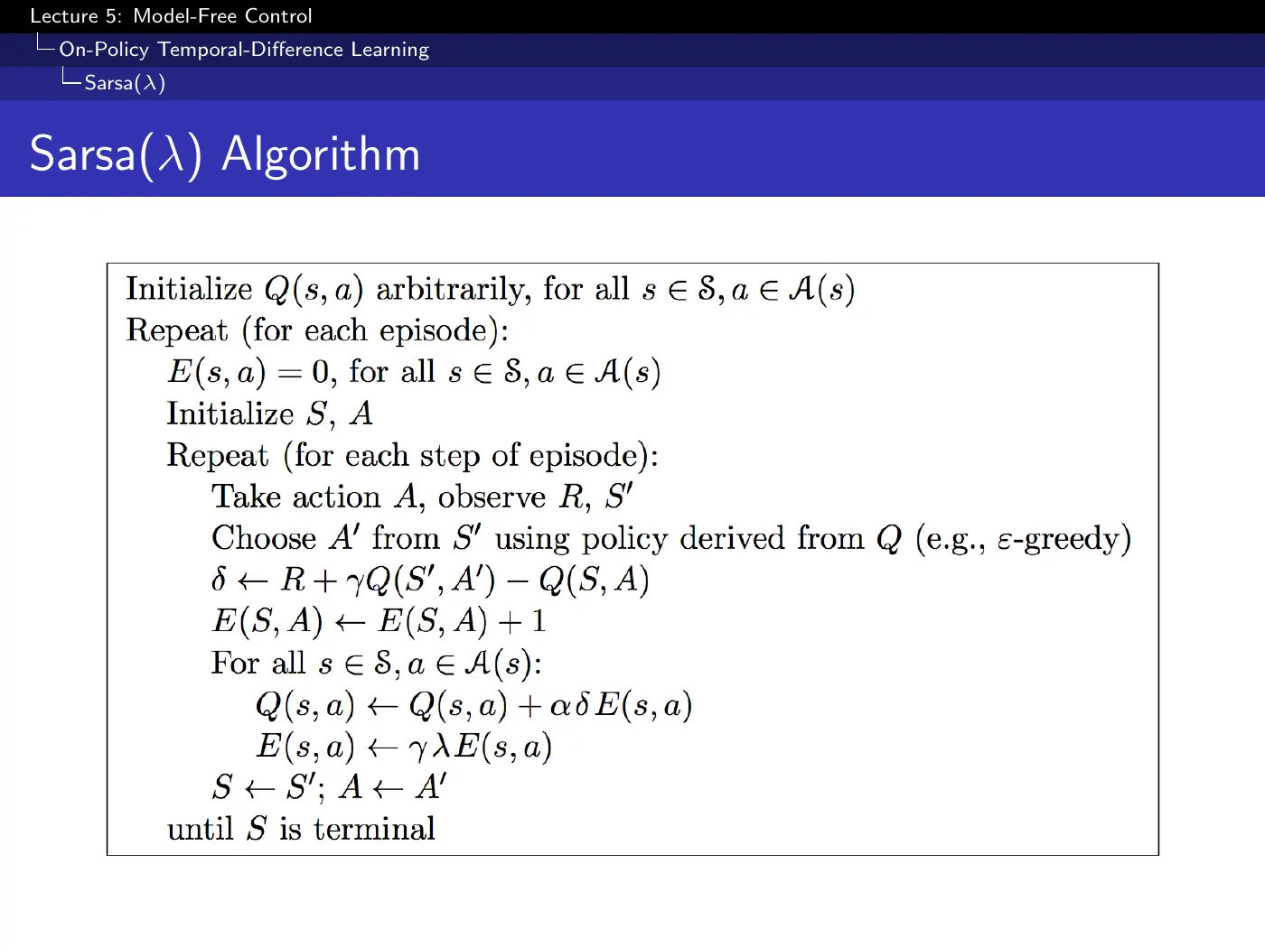
Increment the trace for the one pair you visited. Decay and update every pair in the table, visited or not. Reset $E=0$ at the start of each episode.
Memory cost: $E$ is an $|\mathcal{S}|\times|\mathcal{A}|$ table, the same size as $Q$ — and in L6 both get replaced by function approximators.

p.30 · Sarsa(λ) Gridworld ⏱ 1:06:40

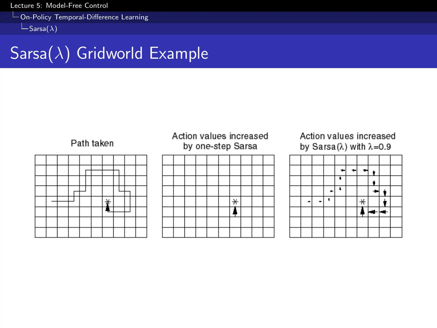
With $Q$ initialized to zero, Sarsa(0) makes almost no progress on the first episode: at every step before the goal, both your estimate and the bootstrapped next estimate are $0$ , so $\delta_t=0$ . Only the final transition carries information. Reward knowledge crawls backward one cell per episode.

Sarsa( $\lambda$ ) has a trace laid along the entire trajectory, so the moment the reward arrives, the whole path updates at once, scaled by each pair's eligibility.

\lambda

defeats the tyranny of the time step

Halve your time-step and Sarsa(0) needs twice as many episodes to propagate the same information. $\lambda$ lets you set how far back credit flows in real time rather than in step count, decoupling the algorithm from your discretization choice.

What this figure does not demonstrate

The advertised benefit of the backward view is that it is online — no waiting for the episode to end. This figure cannot show that, because with a single terminal reward there is genuinely no information to propagate earlier; the updates are running every step, they are just multiplied by $\delta_t=0$ .
The real behavior: with rewards mid-episode, every informative event immediately updates the whole trailing path, without any episode boundary. → Forward and Backward Views of TD Lambda

MC averaged returns explicitly. Where is the average in Sarsa?

There is none. Bootstrapping is a different mechanism for estimating the same expectation — you nudge toward the TD error instead of accumulating a sample mean.
Even substituting $1/N$ for $\alpha$ would not make it a true mean, because the targets themselves keep changing as $Q$ improves. It is a non-stationary average by construction.

7 · Off-policy learning

p.31 · Why bother ⏱ 1:19:42

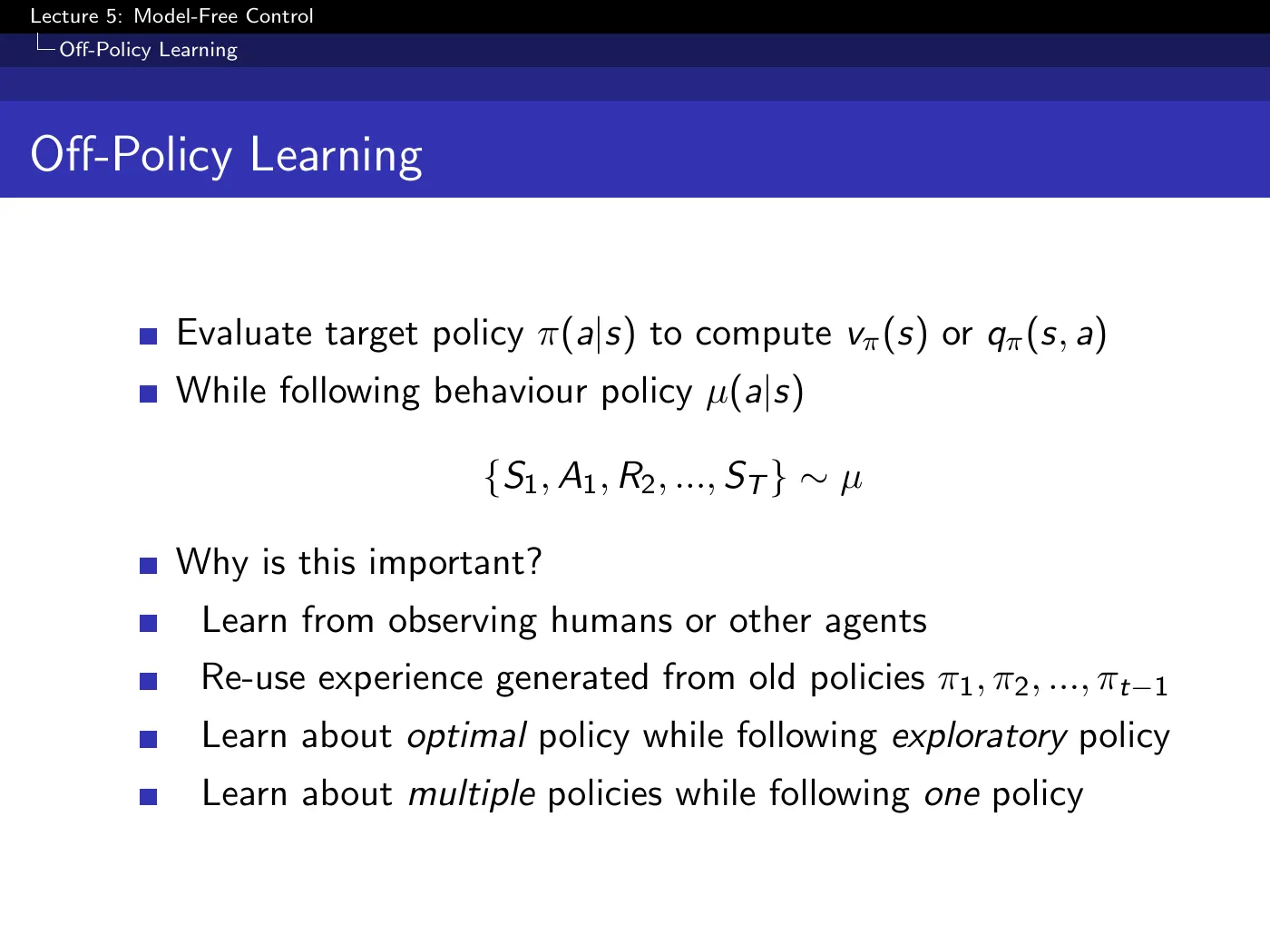
Four motivations, increasing in ambition:

Learn from observing others — humans or other agents — and conclude how to do better than what you observed.
Reuse experience from old policies. GPI marches through $\pi_1,\pi_2,\dots$ ; discarding that data is wasteful. This is the reason off-policy learning is used in the Atari/DQN line of work.
Explore while learning the optimal policy. The best-known use: behave as exploratorily as you like, learn about the deterministic optimum anyway.
Learn about many policies from one stream. "I only get this one stream of data that we call life, and I want to learn about all of these other policies." Answering many counterfactual questions in parallel off a single trajectory.

p.32–33 · Importance Sampling, and why it fails for MC ⏱ 1:25:01

\mathbb{E}_{X\sim P}[f(X)]=\sum_X Q(X)\frac{P(X)}{Q(X)}f(X)=\mathbb{E}_{X\sim Q}\!\left[\frac{P(X)}{Q(X)}f(X)\right]

G_t^{\pi/\mu}=\frac{\pi(A_t|S_t)}{\mu(A_t|S_t)}\cdot\frac{\pi(A_{t+1}|S_{t+1})}{\mu(A_{t+1}|S_{t+1})}\cdots\frac{\pi(A_T|S_T)}{\mu(A_T|S_T)}\;G_t

Why ordinary episode-wise off-policy MC becomes impractical

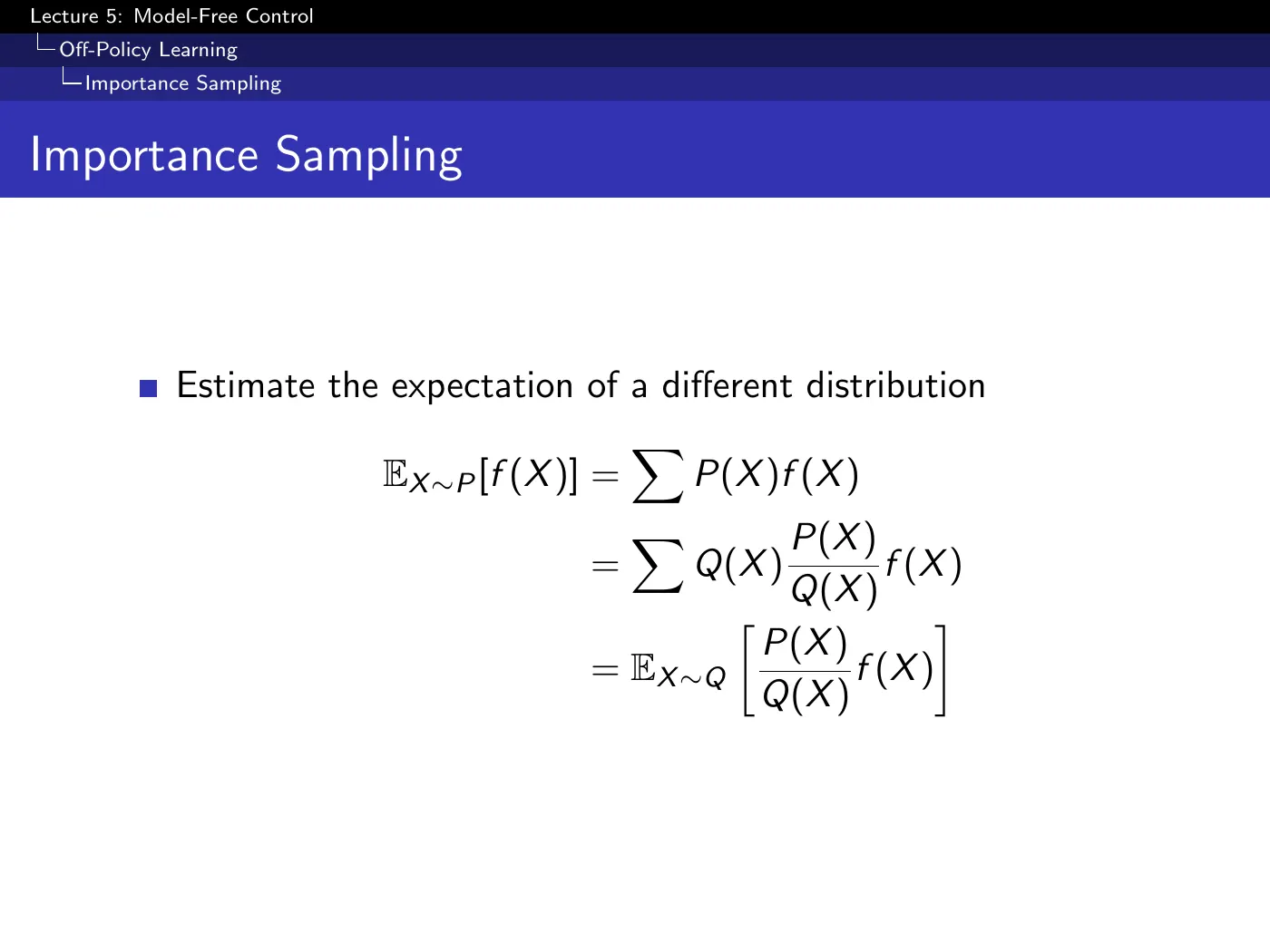
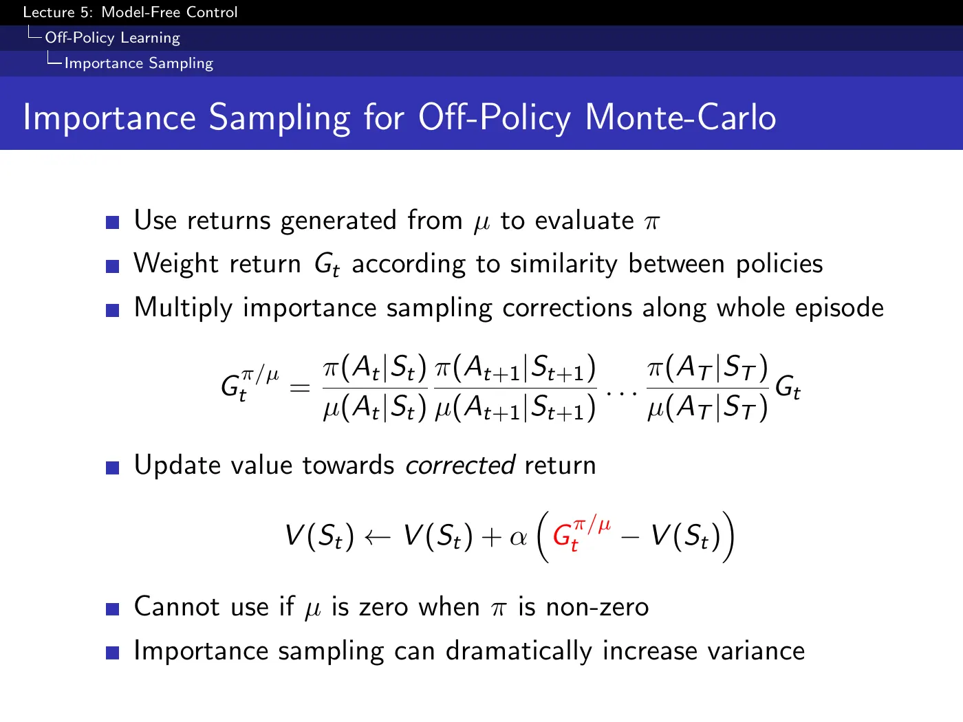
The product does not merely become small. If $\pi$ is deterministic, one action that $\pi$ would never take makes the whole weight zero, while rare fully matching trajectories receive huge weights. The expectation identity remains valid under the support condition, but variance can grow catastrophically.
Silver's “just useless” is a practical verdict for long, substantially different policies, not a theorem that every off-policy MC estimator always fails. Short horizons, similar policies, and weighted or per-decision variants can help. For this lecture's main line, the problem motivates bootstrapping.

p.34 · Importance Sampling for Off-Policy TD ⏱ 1:27:18

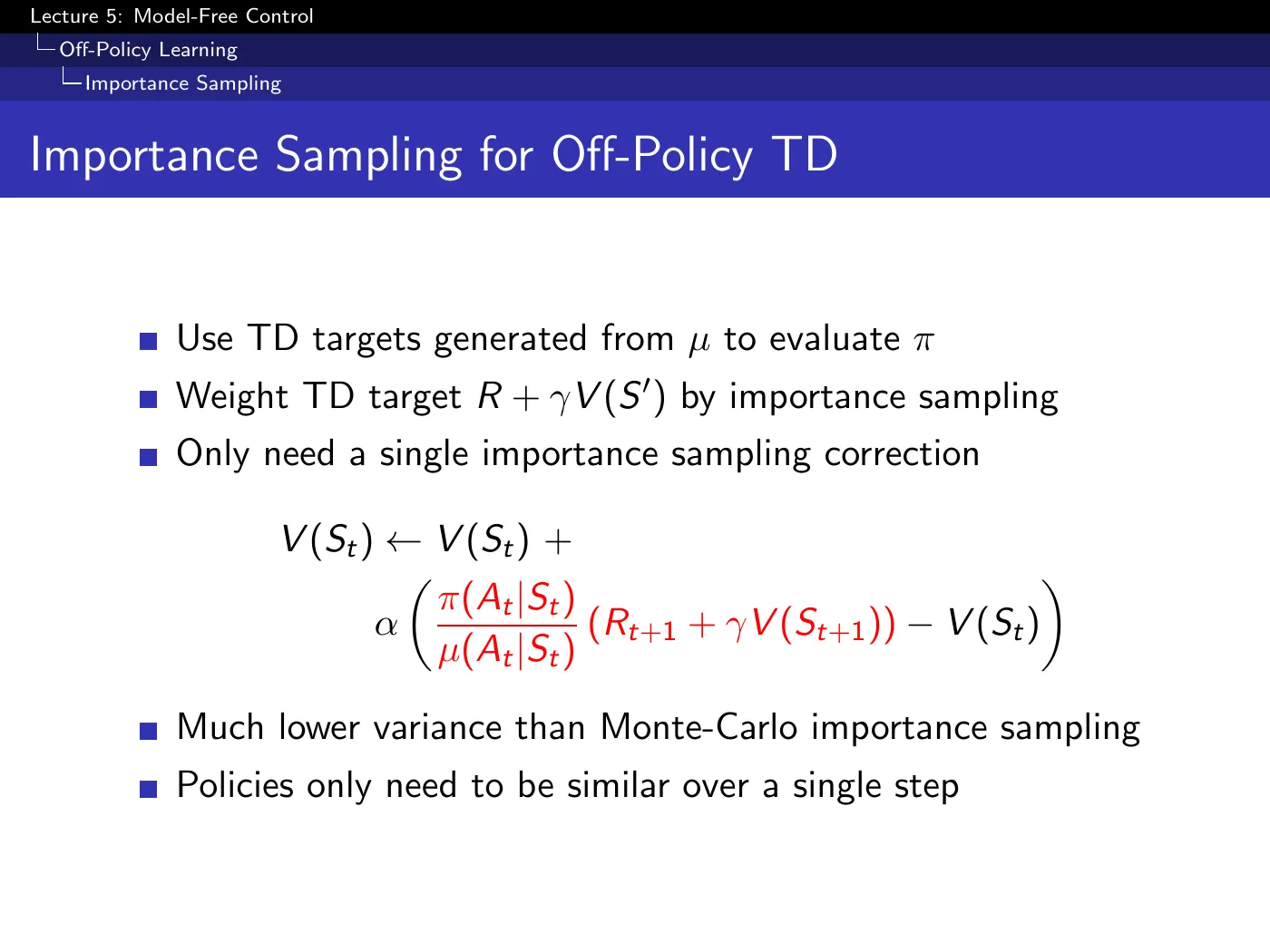
V(S_t)\leftarrow V(S_t)+\alpha\left(\frac{\pi(A_t|S_t)}{\mu(A_t|S_t)}\big(R_{t+1}+\gamma V(S_{t+1})\big)-V(S_t)\right)

Only one correction is needed, because everything past the bootstrap point is already summarized by $V$ . Far lower variance than the MC version — but still capable of blowing up when the two policies disagree on that single step.

Why does the MC ratio product become a rare-event estimator, and why does Q-learning need no ratio? → Importance Sampling in Off-Policy RL

8 · Q-learning

p.35–36 · Off-policy without importance sampling ⏱ 1:28:51

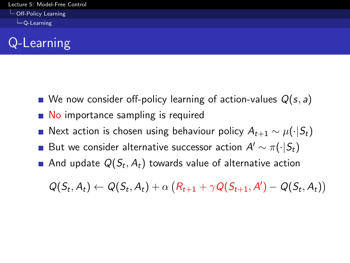
Q(S_t,A_t)\leftarrow Q(S_t,A_t)+\alpha\big(R_{t+1}+\gamma Q(S_{t+1},A')-Q(S_t,A_t)\big), \qquad A_{t+1}\sim\mu(\cdot|S_{t+1}),\quad A'\sim\pi(\cdot|S_{t+1})

The move is to split the action you take from the action you bootstrap from:

Symbol	Drawn from	Used for
$A_{t+1}$	behavior policy $\mu$	actually executed in the environment
$A'$	target policy $\pi$	the bootstrap term only — never executed

Nothing is stored or replayed; both are sampled on the spot. No importance sampling is required because the Bellman equation for $Q$ never asked for it — you are simply sampling a different equation.

Successor-state indexing

The slide conditions $A_{t+1}$ and $A'$ on $S_t$ , but both are successor actions associated with the bootstrap state $S_{t+1}$ . The equations here use $S_{t+1}$ accordingly.

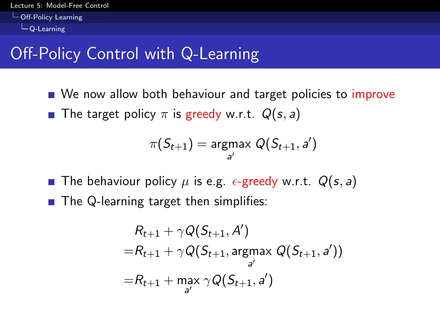
The algorithm everyone calls "Q-learning" is the special case $\pi=$ greedy, $\mu=\epsilon$ -greedy, with both improving over time. Substituting the greedy target collapses the expression:

\gamma Q\big(S_{t+1},\arg\max_{a'}Q(S_{t+1},a')\big)=\gamma\max_{a'}Q(S_{t+1},a')

p.37 · Q-Learning Control Algorithm ⏱ 1:33:27

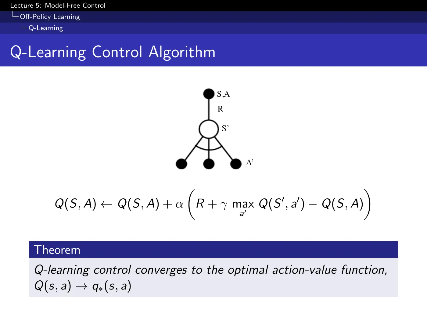
Q(S,A)\leftarrow Q(S,A)+\alpha\Big(R+\gamma\max_{a'}Q(S',a')-Q(S,A)\Big)

Silver's own name for it is the "Sarsamax" update — $S,A,R,S'$ , then a max over $a'$ . It converges to $q_*$ because it samples the Bellman optimality equation, whereas Sarsa samples the expectation equation and converges to $q_\pi$ .

9 · The DP–TD correspondence

p.41–42 ⏱ 1:34:13

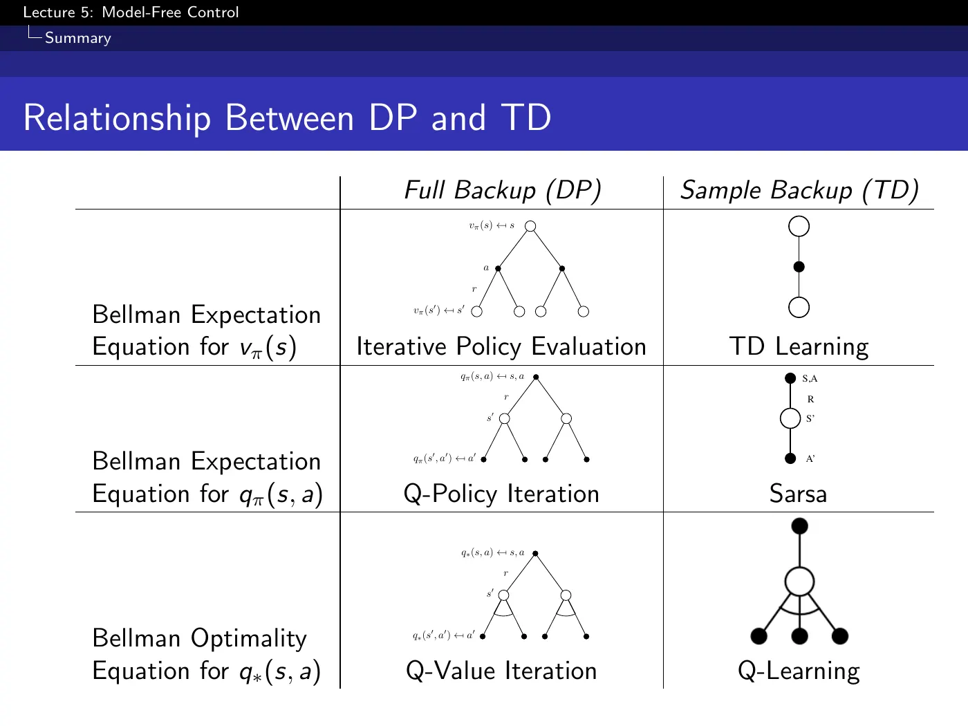
The single sentence this lecture compresses to

A TD target is a sample of the right-hand side of a Bellman equation. DP expands the expectation (full backup); TD samples it (sample backup).

Bellman equation	Full backup (DP)	Sample backup (TD)
expectation for $v_\pi$	iterative policy evaluation	TD learning
expectation for $q_\pi$	Q-policy iteration	Sarsa
optimality for $q_*$	Q-value iteration	Q-learning

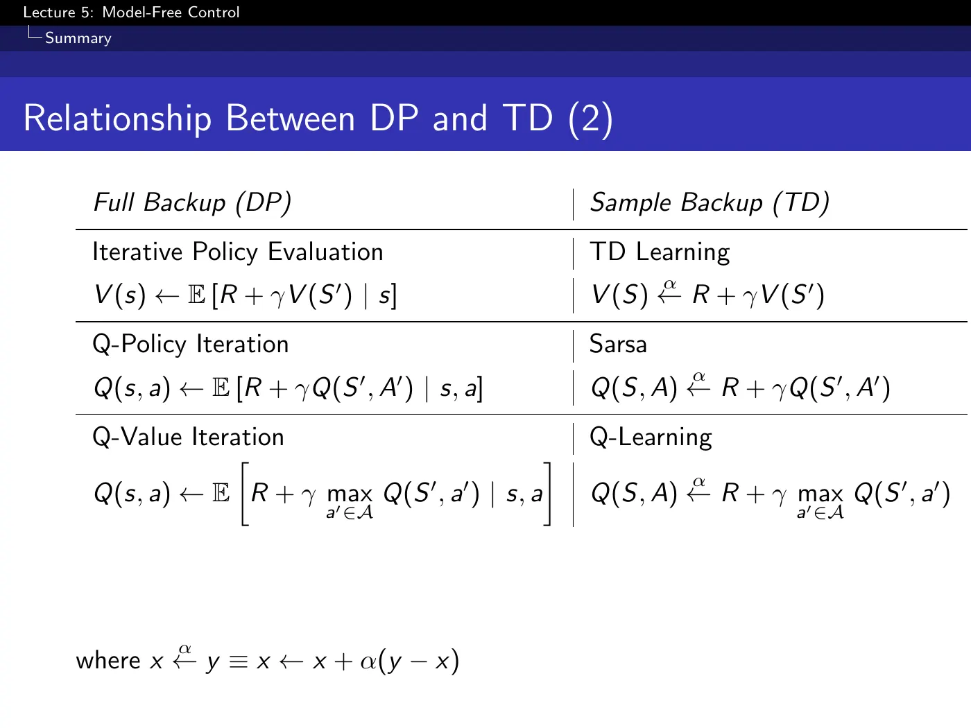
x \xleftarrow{\ \alpha\ } y \quad\equiv\quad x \leftarrow x+\alpha(y-x)

So Sarsa vs. Q-learning is not a matter of algorithmic taste — it is a matter of which Bellman equation you chose to sample. This table is the joint between L3 and L5. → Markov Decision Process (MDP) · Model-Free Prediction

Study checklist

Answer these without the notes before moving on to L6. Each item links back to where it is worked out; open the toggle only after you have tried.

1. Why does greedy improvement on $V$ require a model, and why does $Q$ not?
→ p.8–9 · Model-Free Policy Iteration Using Q ⏱ 9:54

Answer

Greedy on $V$ is $\pi'(s)=\arg\max_a\big(\mathcal{R}^a_s+\gamma\sum_{s'}\mathcal{P}^a_{ss'}V(s')\big)$ — the one-step lookahead is $\mathcal{R}$ and $\mathcal{P}$ , i.e. a model. $Q$ already stores the value of each action separately, so it is a cache of that lookahead: $\pi'(s)=\arg\max_a Q(s,a)$ needs nothing but the table.

2. State the $\epsilon$ -greedy improvement theorem. Which weights make the proof work, and what does the theorem not tell you?
→ p.12 · ε-Greedy Policy Improvement ⏱ 17:31

Answer

For any $\epsilon$ -greedy policy $\pi$ , the $\epsilon$ -greedy policy $\pi'$ with respect to $q_\pi$ satisfies $v_{\pi'}\ge v_\pi$ .
The proof is one inequality — a max dominates any convex combination — and the weights that make it collapse are $w_a=\dfrac{\pi(a|s)-\epsilon/m}{1-\epsilon}$ . With those, the $1-\epsilon$ factors cancel and the remainder is exactly $\sum_a\pi(a|s)q_\pi(s,a)=v_\pi(s)$ .
What it does not give you: any guidance on how much to explore or how fast $\epsilon$ should decay. Monotone improvement holds for any fixed $\epsilon$ — and a fixed $\epsilon$ never reaches $q_*$ . That is GLIE's job, not this theorem's. It is also a one-step result; $v_{\pi'}\ge v_\pi$ needs the L3 telescoping argument on top.

3. What are the two GLIE conditions, and what specifically goes wrong if you drop the second?
→ p.15 · GLIE ⏱ 25:15

Answer

(i) $\lim_{k\to\infty}N_k(s,a)=\infty$ — every pair is visited infinitely often, or its estimate stays wrong forever.
(ii) $\lim_{k\to\infty}\pi_k(a|s)=\mathbf{1}\big(a=\arg\max_{a'}Q_k(s,a')\big)$ — the policy becomes greedy in the limit.
Drop (ii) and you still converge, just to the wrong thing: a permanently soft policy satisfies the Bellman expectation equation for that soft policy, so you get $q_\pi$ of your $\epsilon$ -soft policy. The optimality equation contains a $\max$ , and only a policy going greedy in the limit samples it.

4. Why is the MC control average not an i.i.d. mean, and why does it converge anyway?
→ p.16 · GLIE Monte-Carlo Control ⏱ 28:17

Answer

The returns being averaged into $Q(S_t,A_t)$ come from a sequence of different policies — $\pi$ improves after every episode — so they are not identically distributed.
GLIE rescues it: as $\pi_k$ approaches greedy, the early samples generated by bad policies are progressively dominated by the later ones, and the running average converges on $q_*$ .

5. Why is Sarsa on-policy by construction rather than by convention?
→ p.22 · Sarsa Algorithm ⏱ 44:29

Answer

The target $R+\gamma Q(S',A')$ is a sample of the Bellman expectation equation for $q_\pi$ , whose right-hand side is two expectations: $R,S'$ over the environment, and $Q(S',A')$ over your own policy from $S'$ onward. That second term is the quantity being estimated, so $A'$ must be drawn from the policy under evaluation or the target is not a sample of the right thing.
Breaking that constraint is exactly what Q-learning does — and it has to switch to a different Bellman equation to stay valid.

6. Why does Sarsa(0) propagate reward information only one cell per episode?
→ p.30 · Sarsa(λ) Gridworld ⏱ 1:06:40

Answer

With $Q$ initialized to zero and a single terminal reward, every step before the goal has $Q(S,A)=0$ and $Q(S',A')=0$ , so $\delta_t=0$ — the update runs but multiplies by nothing. Only the final transition carries information, so episode 1 updates exactly one pair. Each subsequent episode moves that frontier back by one cell.
Sarsa( $\lambda$ ) has a trace laid along the whole trajectory, so when the reward arrives the entire path updates at once, scaled by each pair's eligibility.

7. What does " $\lambda$ defeats the tyranny of the time step" mean concretely?
→ p.30 · Sarsa(λ) Gridworld ⏱ 1:06:40

Answer

Sarsa(0) propagates credit one cell per step count, so halving your discretization doubles the number of episodes needed to move the same information the same real distance — the algorithm's behavior is hostage to an arbitrary modeling choice.
The trace decays by $\gamma\lambda$ per step, so $\lambda$ sets how far back credit flows in real time, and you can hold that horizon fixed while changing the time-step.

8. Why is off-policy MC with importance sampling unusable, and what does that force you to do instead?
→ p.32–33 · Importance Sampling, and why it fails for MC ⏱ 1:25:01

Answer

The weight is a product of per-step ratios over the entire episode. If $\pi$ is deterministic, a single action it would never take zeroes the whole weight, while the rare fully matching trajectories get enormous weights — a rare-event estimator whose variance can grow catastrophically. (The identity itself stays valid under the support condition; "useless" is a practical verdict for long, substantially different policies, not a theorem.)
It forces you to bootstrap: TD needs only one ratio per step (p.34), and Q-learning removes the ratio entirely. → Importance Sampling in Off-Policy RL

9. Why does Q-learning need no importance sampling?
→ p.35–36 · Off-policy without importance sampling ⏱ 1:28:51

Answer

Because it never reweights anything. It splits the action taken from the action bootstrapped from: $A_{t+1}\sim\mu$ is executed, $A'\sim\pi$ appears only in the target and is sampled on the spot. You are not correcting $\mu$ 's samples into an expectation under $\pi$ — you are sampling a different Bellman equation, the optimality equation, whose right-hand side asks for $\max_{a'}Q(S_{t+1},a')$ and nothing about $\mu$ .

10. Reconstruct the DP–TD table from memory.
→ 9 · The DP–TD correspondence

Answer

A TD target is a sample of the right-hand side of a Bellman equation. DP expands the expectation (full backup); TD samples it (sample backup).

Bellman equation	Full backup (DP)	Sample backup (TD)
expectation for $v_\pi$	iterative policy evaluation	TD learning
expectation for $q_\pi$	Q-policy iteration	Sarsa
optimality for $q_*$	Q-value iteration	Q-learning

Gaps to close on your own

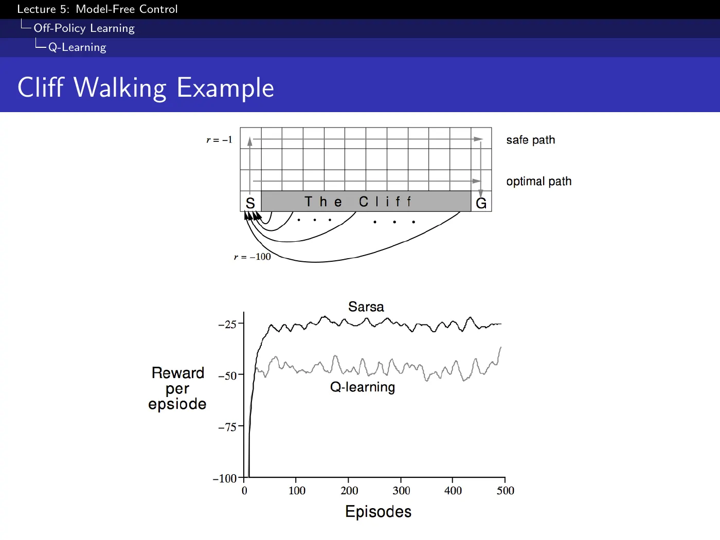
Slides p.38–40 are skipped in the lecture

The video jumps from p.37 straight to the summary, leaving three slides unexplained — the Q-learning pseudocode, the demo, and Cliff Walking.
Cliff Walking is the standard demonstration of the practical difference between Sarsa and Q-learning: the on-policy learner walks the safe route away from the edge, the off-policy learner learns the optimal edge-hugging path but performs worse online because

\epsilon

occasionally knocks it off. Working through it is the fastest way to make the on/off-policy distinction concrete.

Windy Gridworld move set — the lecture is ambiguous about whether the figure uses the four standard moves or king's moves (diagonals). Sutton & Barto Example 6.5 is the reference; confirm there before quoting the numbers.
Forward/backward equivalence for the control case is asserted, not proved. The L4 proof is said to carry over → Forward and Backward Views of TD Lambda.
Function approximation — everything here is a lookup table, which does not scale. That is L6, and it applies to $E$ as well as $Q$ .

Language notes

Phrasings worth stealing for your own technical writing and talks:

Expression	Use
learn on the job / look over someone's shoulder	naming on- vs off-policy without formalism
vanishingly small	a quantity decaying toward zero, informally but precisely
let me back off that	retracting a claim mid-sentence without losing authority
it defeats the tyranny of the time step	a design choice removing a dependence on an arbitrary parameter
a thorny problem	genuinely hard and unresolved, not merely difficult
get the best of both worlds	a method inheriting the advantages of two extremes
this is naive but surprisingly hard to beat	conceding simplicity while defending a baseline

The one idea

Contents

1 · Why model-free control

p.4 · Uses of Model-Free Control ⏱ 2:17

p.5 · On- and Off-Policy Learning ⏱ 3:47

2 · Making GPI model-free

p.6–7 · Generalized Policy Iteration ⏱ 5:18

p.8–9 · Model-Free Policy Iteration Using Q ⏱ 9:54

3 · Exploration and ε-greedy

p.10 · Example of Greedy Action Selection ⏱ 12:56

p.11 · ε-Greedy Exploration ⏱ 15:13

p.12 · ε-Greedy Policy Improvement ⏱ 17:31

4 · GLIE Monte-Carlo control

p.13–14 · Monte-Carlo Policy Iteration → Control ⏱ 22:04

p.15 · GLIE ⏱ 25:15

p.16 · GLIE Monte-Carlo Control ⏱ 28:17

p.17–18 · Blackjack ⏱ 34:39

5 · Sarsa

p.19 · MC vs. TD Control ⏱ 38:26

p.20–21 · The Sarsa Update ⏱ 39:57

p.22 · Sarsa Algorithm ⏱ 44:29

p.23 · Convergence of Sarsa ⏱ 48:14

p.24–25 · Windy Gridworld ⏱ 49:46

6 · Sarsa(λ)

p.26 · n-Step Sarsa ⏱ 53:40

p.27 · Forward View ⏱ 56:43

p.28–29 · Backward View ⏱ 1:00:30

p.30 · Sarsa(λ) Gridworld ⏱ 1:06:40

7 · Off-policy learning

p.31 · Why bother ⏱ 1:19:42

p.32–33 · Importance Sampling, and why it fails for MC ⏱ 1:25:01

p.34 · Importance Sampling for Off-Policy TD ⏱ 1:27:18

8 · Q-learning

p.35–36 · Off-policy without importance sampling ⏱ 1:28:51

p.37 · Q-Learning Control Algorithm ⏱ 1:33:27

9 · The DP–TD correspondence

p.41–42 ⏱ 1:34:13

Study checklist

Gaps to close on your own

Language notes