Lecture 10 · Classic Games

Slides: David Silver - RL Course (UCL 2015) · Previous: Lecture 9 · Exploration and Exploitation · Next: — (final lecture)

First pass: read The one idea and the slide-group headings. Use the prose when an equation, condition, or figure needs explanation; leave Gaps to close for review.

This is the lecture where the slides matter most, and the video shows them worst

L10 is a case-study lecture: the payload is in tables, game positions, and search-tree diagrams, and the recording makes several of them hard to read. Everything below is embedded from the source PDF at full resolution, so the figures you could not make out in the video are legible here.

The one idea

Nine lectures built machinery. This one asks a single question: when people actually beat world champions, what did they use? — and the answer turns out to be one recipe, applied seven times.

The final slide is the whole lecture:

	Input features	Value fn	RL	Training	Search
Chess (Meep)	binary	linear	TreeStrap	self-play	$\alpha\beta$
Checkers (Chinook)	binary	linear	TD leaf	self-play	$\alpha\beta$
Othello (Logistello)	binary	linear	MC	self-play	$\alpha\beta$
Backgammon (TD-Gammon)	binary	neural net	TD( $\lambda$ )	self-play	$\alpha\beta$ / MC
Go (MoGo)	binary	linear	TD	self-play	MCTS
Scrabble (Maven)	binary	linear	MC	self-play	MC search
Poker (SmooCT)	binary	linear	MCTS	self-play	—

Read the columns, not only the rows. A repeated pattern appears: compact binary features, often a linear value function, self-play, and search. The exact learning and search algorithms vary by game, and TD-Gammon's neural network is the clearest representation outlier.

The recurring three-part recipe

Self-play can supply the data without a fixed expert dataset, by letting the agent adapt to opponents that are also changing.
A value function compresses what was learned into a position evaluation.
Search recovers, at play time, the tactical precision the value function cannot represent.
These are not logical necessities for every game — Deep Blue had no learning, and some table entries use little or no online search. They are the recurring empirical recipe behind the RL systems in this lecture.

Nash equilibrium is a fixed point of self-play, which is why self-play is principled

A best response to fixed opponents is an ordinary single-agent RL problem — push the opponents into the environment and solve the resulting MDP. A Nash equilibrium is the joint policy where everyone is simultaneously playing a best response.
Self-play aims at that condition: each player's policy defines the other's environment, so improving one changes the problem the other faces. If every player is a best response at a fixed point, that fixed point is a Nash equilibrium. Reaching such a point is not automatic; naive best-response dynamics can cycle.

1 · Why games, and where the state of the art stands
2 · Game theory, minimally
3 · Minimax search
4 · Self-play reinforcement learning
5 · TD-Gammon
6 · Learning from search values
7 · Simulation-based search
8 · Imperfect information
9 · The recipe, and the assumption that broke
Study checklist
Gaps to close on your own
Language notes

1 · Why games, and where the state of the art stands

p.3–5 · Why Study Classic Games ⏱ 2:22

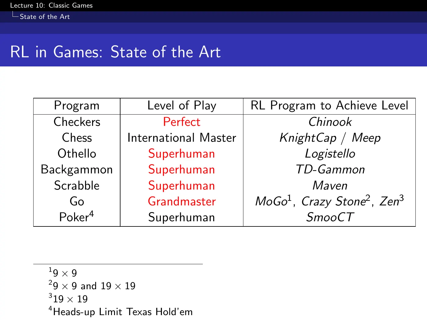
Chess was called the Drosophila of AI — the fruit fly, the organism simple enough to run thousands of experiments on while still exhibiting the phenomena you care about. That is the honest case for games: simple enough to iterate, deep enough to matter, and with a benchmark no other domain offers — humans who have spent their lives becoming the best possible at exactly this.

Compare p.4 (all of AI) against p.5 (RL only) and read the overlap: five of seven games were first brought to their best-known level by reinforcement learning. The two exceptions are instructive rather than embarrassing — in chess RL reached International Master, well short of Deep Blue, and in poker there is now a superhuman RL method.

That is the claim underwriting the rest of the lecture: RL is not one approach among many here. It is the primary mechanism by which classic games were solved.

2 · Game theory, minimally

p.6–7 · Best Response and Nash Equilibrium ⏱ 7:41

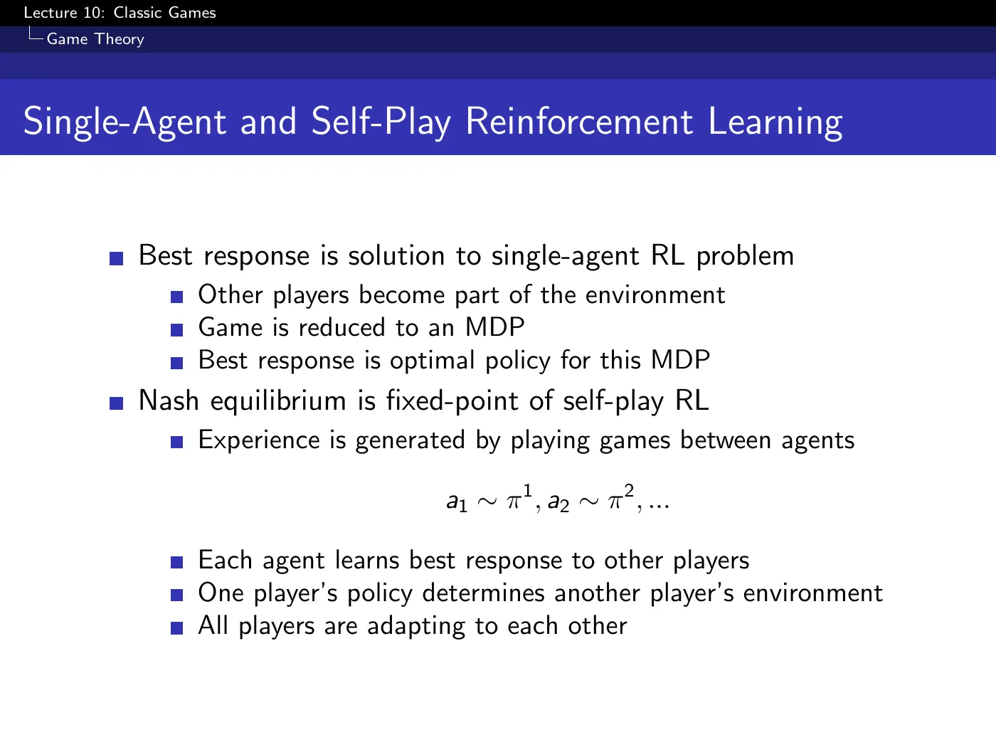
In an MDP "optimal" is unambiguous. With another player it is not: the best policy against an opponent who always plays rock is to always play paper, and that policy is catastrophic against anyone else. Optimality has to be defined relative to what everyone else does, which is why the lecture needs game theory at all.

Two concepts, and the second is the one that matters:

Best response $\pi^i_*(\pi^{-i})$ — the optimal policy against fixed opponents. Push them into the environment and it is an ordinary MDP.
Nash equilibrium — a joint policy where every player is playing a best response to all the others. Nobody would choose to deviate.

For rock-paper-scissors the Nash equilibrium is uniform random. Any deviation creates a regularity, and a regularity is exploitable.

Is the Nash equilibrium unique?

Not in general. In the two-player zero-sum setting, the minimax value is unique, but multiple policies can attain it; therefore equilibrium policies need not be unique even when the value is. The slide makes the precise claim: a minimax policy is a Nash equilibrium and the minimax value function is unique.
Imperfect-information games such as poker can also have many equilibrium strategies. Section 8 needs different machinery primarily because players act from different information states, not merely because equilibria may be non-unique.

The connection back to your own homework

Easy21 fixed the dealer's policy and folded it into the environment — a best-response problem. If both sides learn and the process reaches an equilibrium, the result is a joint solution concept rather than a policy tailored to one fixed dealer. Convergence still depends on the particular multi-agent algorithm and its assumptions.

The convergence question is deferred until ⏱ 1:24:33. Silver points to Littman's tabular minimax-RL results as evidence that convergence is possible for suitable algorithms and assumptions. Do not generalize this to arbitrary “standard RL under self-play”; everything practical in this lecture uses approximation or search outside that simple guarantee.

p.8–9 · Zero-Sum and Perfect Information ⏱ 18:20

Two restrictions, each buying something concrete:

Zero-sum ( $R^1+R^2=0$ ) means good-for-white is exactly bad-for-black, so one value function suffices — negate it for the other player's view. It also means the players are never partly cooperating, which is what makes minimax the right solution concept.

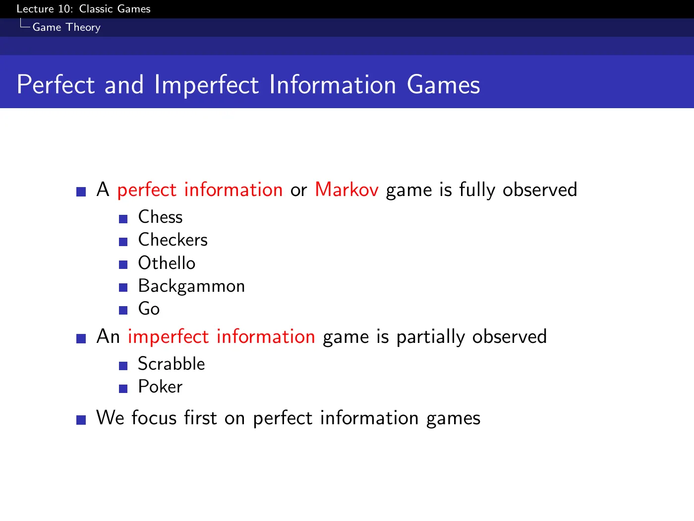
Perfect information means fully observed. Note that this does not mean deterministic: backgammon has dice and is still perfect information, because you see the entire board state. The distinction is observability, not stochasticity — a confusion the slide's bullet list invites.

3 · Minimax search

p.10–11 · The Minimax Value Function ⏱ 21:23

v_*(s)=\max_{\pi^1}\min_{\pi^2}v_\pi(s)

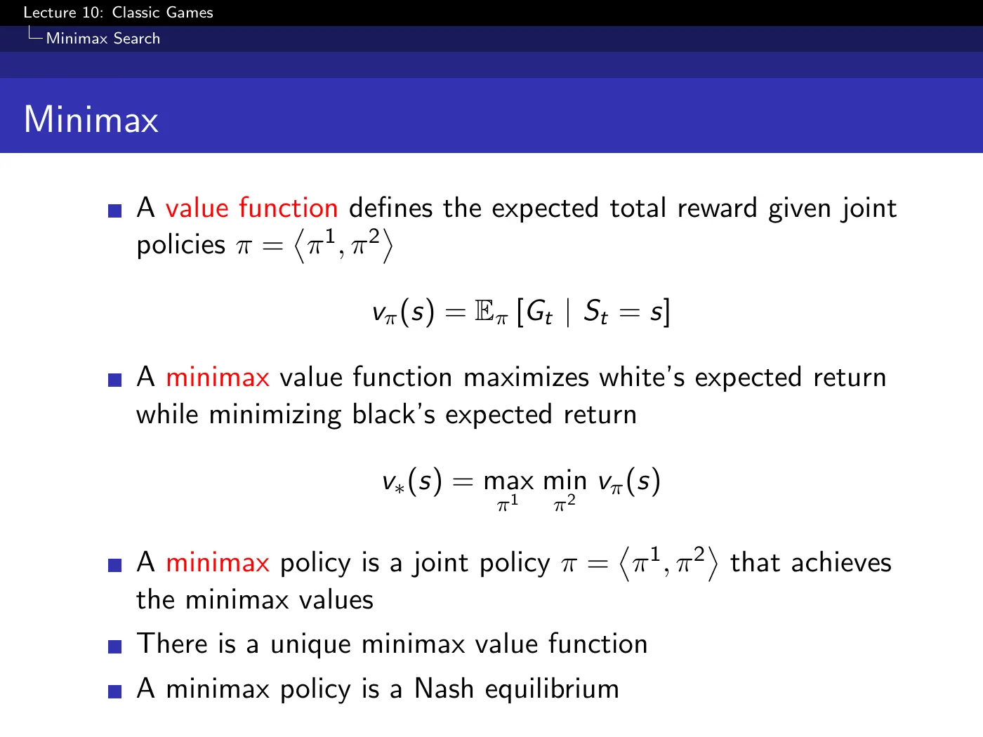
Read it as "if both players try their hardest against each other, who wins from here?" The $\max\min$ notation compresses a nested alternation — white maximizes, then black minimizes, then white maximizes — down the whole sequence. It is shorthand for the tree, not a two-step operation.

In the standard game setting there are no intermediate rewards: zero throughout, then a terminal outcome. If the payoff is $1$ for a win and $0$ otherwise, $v_\pi(s)=\mathbb P(\text{win}\mid s)$ . With $+1$ for a win and $-1$ for a loss and no draws,

v_\pi(s)=2\,\mathbb P(\text{win}\mid s)-1.

So value is an affine transform of win probability, not literally the probability under every reward convention.

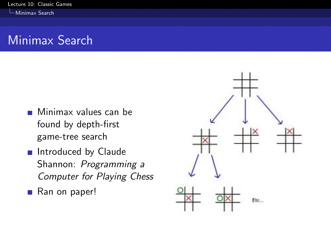
Minimax search dates to Claude Shannon's Programming a Computer for Playing Chess — the first chess program ever written, which ran on paper, because there was no computer to run it on. Most of the concepts still in use were already there.

p.12–15 · The Worked Example ⏱ 27:29

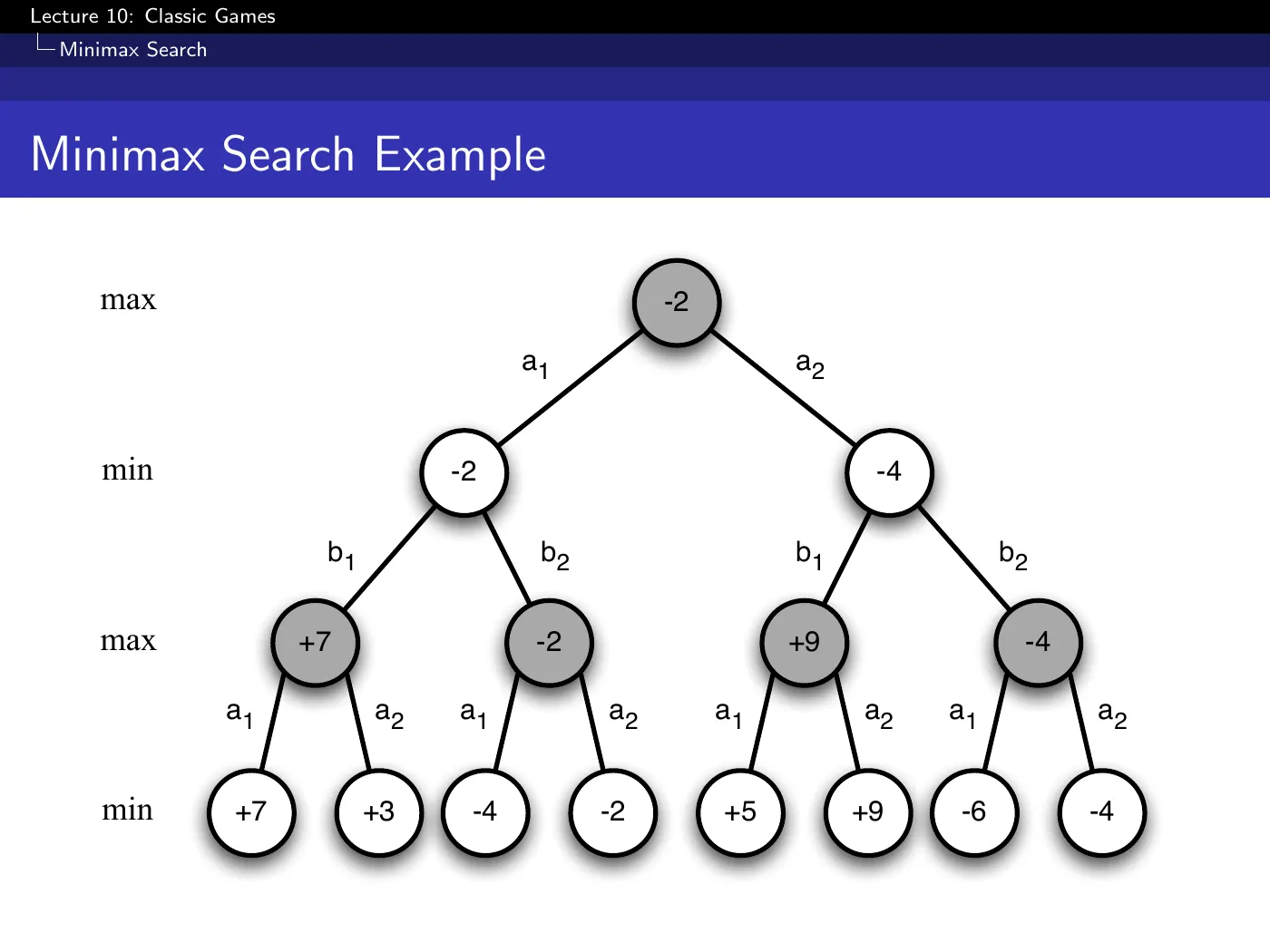
Four slides animating one depth-first pass: evaluate the leaves, take maxima at Max's nodes, minima at Min's, and back up to the root, which comes out at $-2$ via $a_1$ .

The thing to extract is not the arithmetic but the consequence: this computes the optimal policy, not just the optimal values. The backed-up choice at each node is the minimax policy. If you could run this to the end of the game you would be finished.

You cannot, because the tree grows exponentially with depth. Everything after this slide is a response to that one fact.

p.16–17 · Truncating the Search with a Value Function ⏱ 29:45

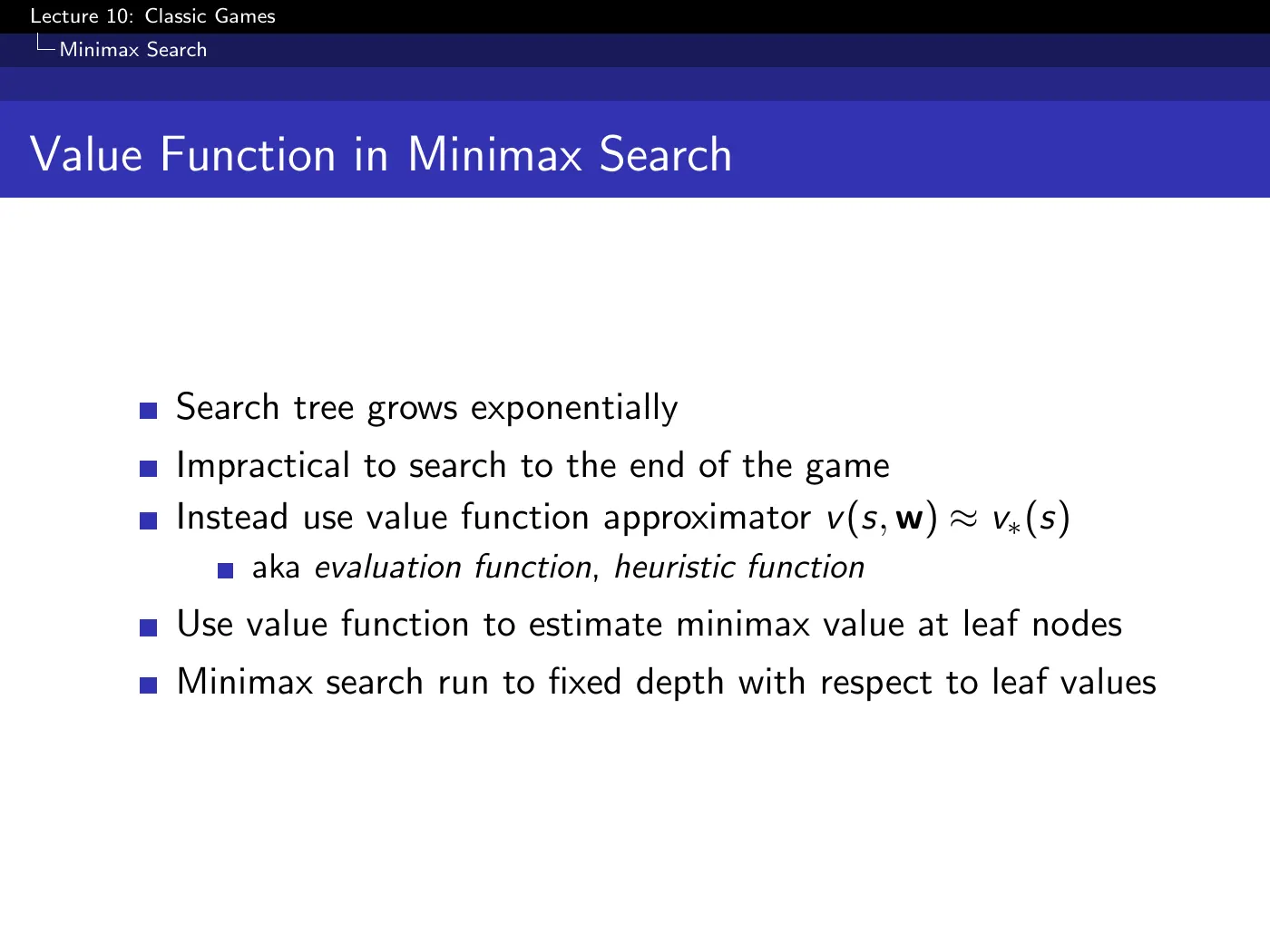
Search to a fixed depth, then call a function approximator at the leaves and back those values up instead of real outcomes.

The evaluation function is a value function, and naming it correctly is the point

Game-tree literature calls it an "evaluation function" or "heuristic function", which makes it sound like a domain-specific device. In this course's vocabulary it is exactly $\hat v(s,\mathbf{w})\approx v_*(s)$ — a value function approximator estimating the minimax value.
Once you see that, the whole of L6 applies to it, and the rest of the lecture becomes "how do we learn these weights?" rather than "what heuristic should we hand-write?".

v(s,\mathbf{w})=x(s)\cdot\mathbf{w}=5+3-5=3

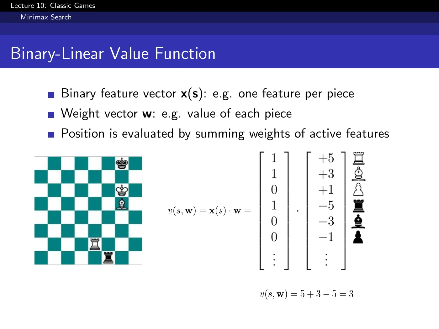
The binary-linear evaluation is the same construction from L6 p.15 — binary features, a weight per feature, and a dot product. What makes it fast is sparsity: you never touch the zero features; you sum the weights of the features that are present.

Two extensions the slide does not mention. Piece-square tables condition a piece's value on where it sits, and modern programs use conjunctions of pieces and positions — a strong shogi program uses on the order of ten million such features. The construction does not change; only the feature count does.

The resulting score need not be a calibrated win probability. A logistic output can enforce a probability-like range, but many game engines use an uncalibrated evaluation scale because search needs reliable ordering more than calibrated probabilities.

p.18–19 · Deep Blue and Chinook ⏱ 35:48

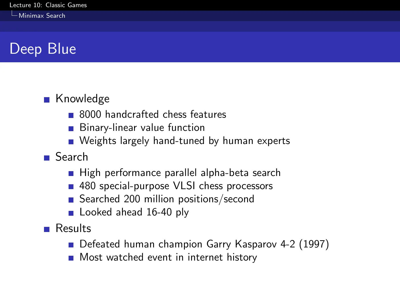
Deep Blue contains no learning at all

8,000 handcrafted features with weights hand-tuned by a team of human grandmasters, plus 480 custom chess processors searching 200 million positions per second, 16–40 ply deep. It defeated Kasparov 4–2 in 1997.
It is in this lecture as the null hypothesis: this is what pure search plus pure human knowledge achieves. Every RL result afterwards is measured against the fact that it needed no grandmasters.
A footnote on the history: Kasparov was rattled by playing a machine and blundered uncharacteristically, and computer chess arguably needed another few years to be genuinely stronger. The 1997 date marks the perception, not quite the crossing.

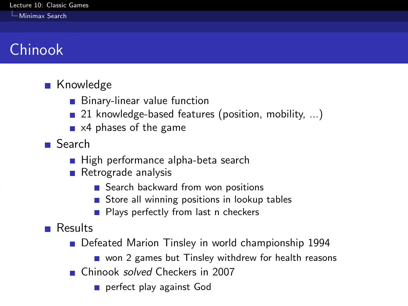
Chinook's retrograde analysis is a second search running the other way: start from won positions, work backwards, and tabulate every position from which a win is forced. With 11 or fewer pieces on the board, Chinook stopped searching and simply looked up the answer.

The Tinsley story is worth knowing. Marion Tinsley lost seven games in his entire career; two were to Chinook, in a championship match he had to abandon for health reasons before dying. Unable to settle it against the best human, Jonathan Schaeffer settled it against the best possible play instead — solving checkers outright in 2007, roughly $10^{24}$ positions.

The reason two search-only systems open a reinforcement learning lecture

It is a corrective, stated outright: it is easy to slip into believing you learn a value function or a network and then just apply it. In these domains search is the primary driver of performance, and you must evaluate the position in front of you dynamically. The rest of the lecture is about combining the two, not replacing one with the other.

4 · Self-play reinforcement learning

p.20–21 · Self-Play TD and Afterstates ⏱ 42:38

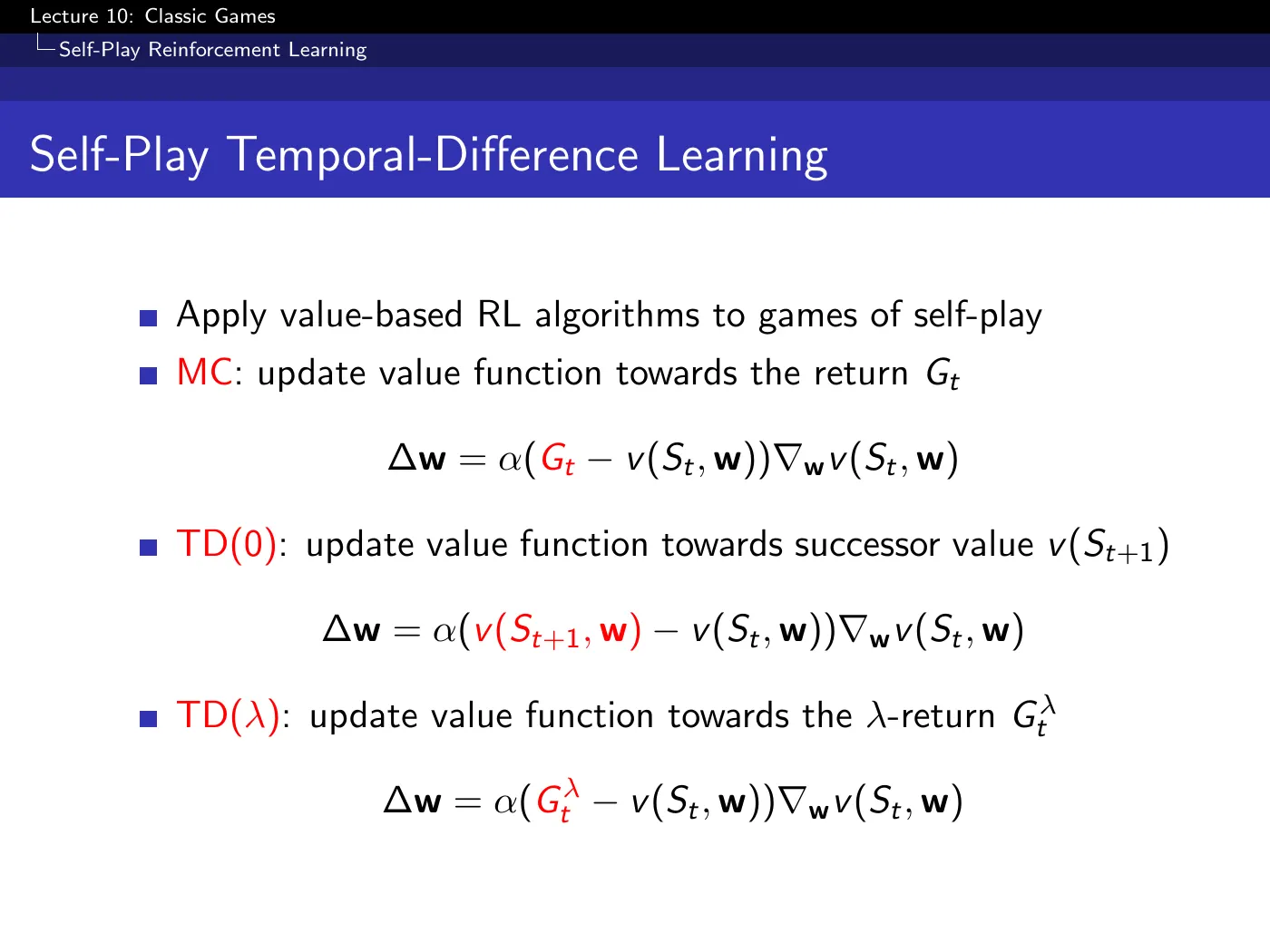
\Delta\mathbf{w}=\alpha\big(v(S_{t+1},\mathbf{w})-v(S_t,\mathbf{w})\big)\nabla_\mathbf{w}v(S_t,\mathbf{w})

Almost nothing changes. On non-terminal transitions the TD update is the L6 update with an immediate reward of zero. At the terminal transition, the win/loss outcome supplies the target. Code still needs this terminal boundary condition even though the displayed interior update has no reward term.

Two things do change, and neither is on the slide:

You are estimating minimax values, not $v_\pi$ for a fixed policy.
Policy improvement improves both players at once — maximizing for white and minimizing for black — which is what drives the pair toward equilibrium rather than toward one player exploiting the other.

q_*(s,a)=v_*(\text{succ}(s,a))

Afterstates dissolve the reason L5 needed

Q

at all

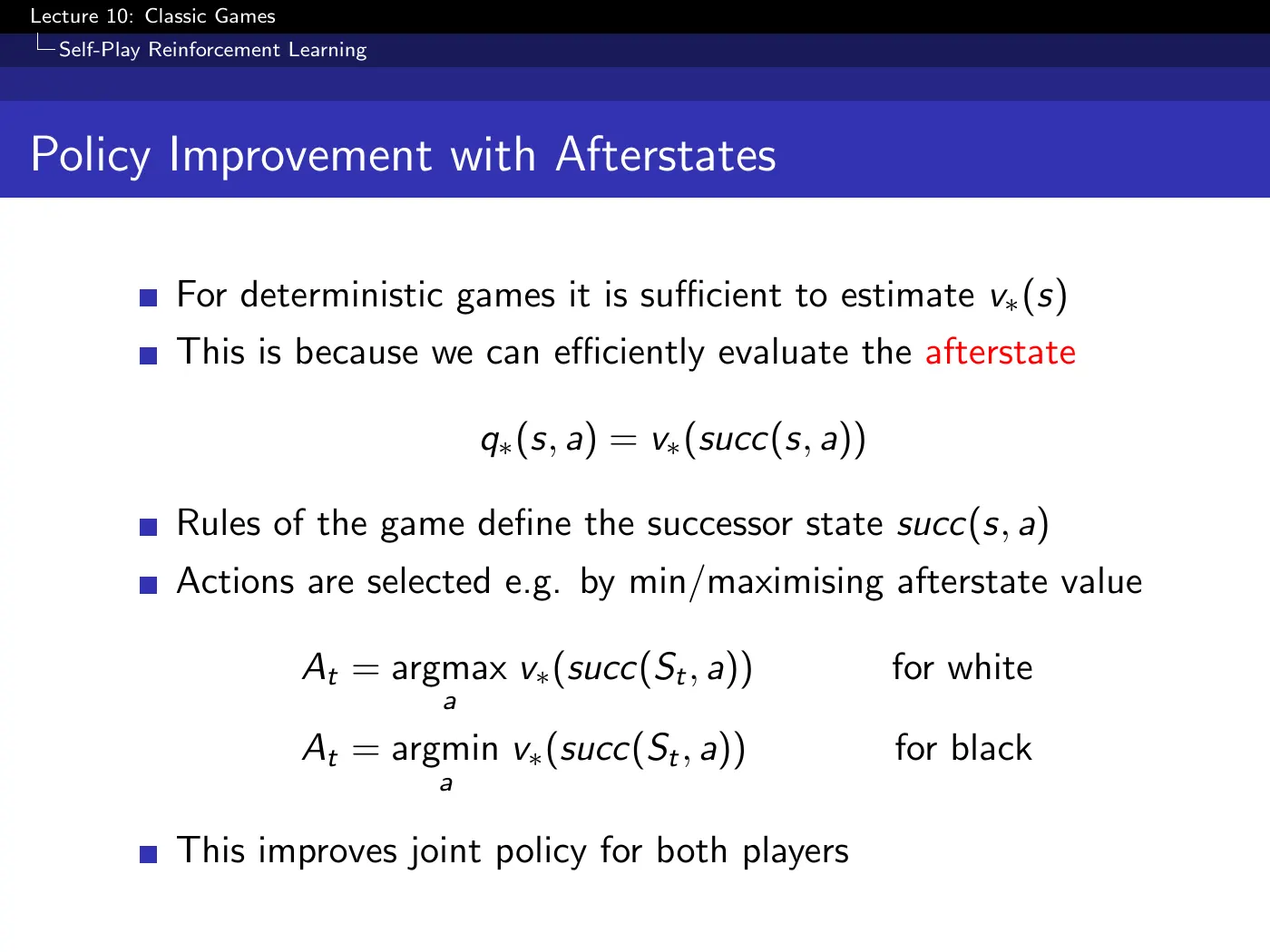
L5's whole first substitution was $V\to Q$ , because greedy improvement on $V$ needs a model. In a deterministic game you have the model — it is the rules — so $\text{succ}(s,a)$ is free, and $q_*$ reduces to $v_*$ evaluated at the resulting position.
The saving is real: instead of a table over $|\mathcal{S}|\times|\mathcal{A}|$ you keep one over positions, and many action sequences that transpose to the same position share an entry automatically.
The precondition is deterministic transitions plus known rules. It fails the moment either does.

p.22–23 · Logistello ⏱ 47:10

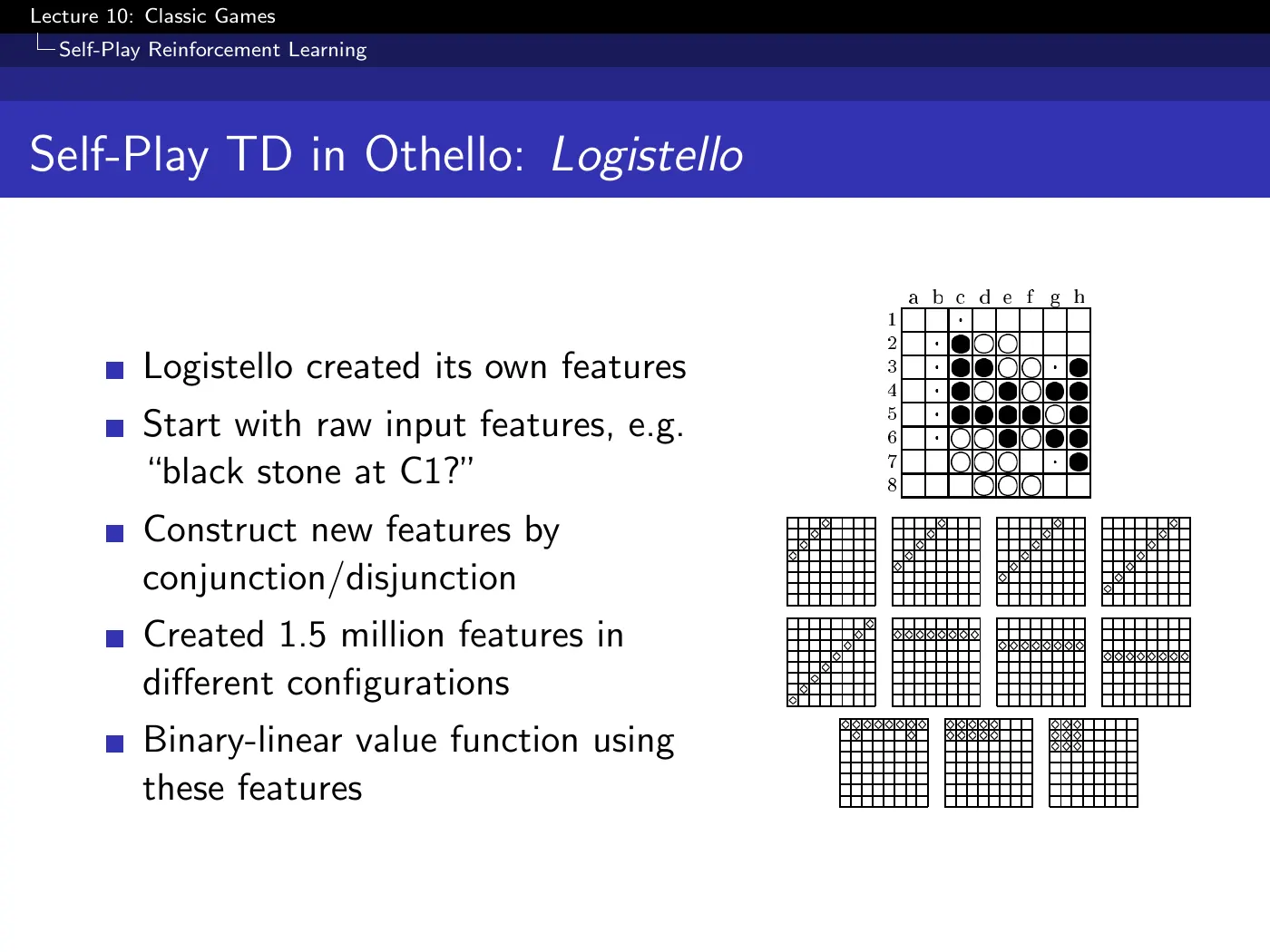
Deep Blue's features were written by grandmasters. Logistello's were discovered by the program: take raw features like "black stone at C1", form conjunctions and disjunctions within pattern templates that matter in Othello (corners, diagonals, lines), and keep the configurations that actually occur in self-play games. That produced 1.5 million binary features.

The only prior knowledge injected is which regions of the board to build patterns over. Everything else is learned.

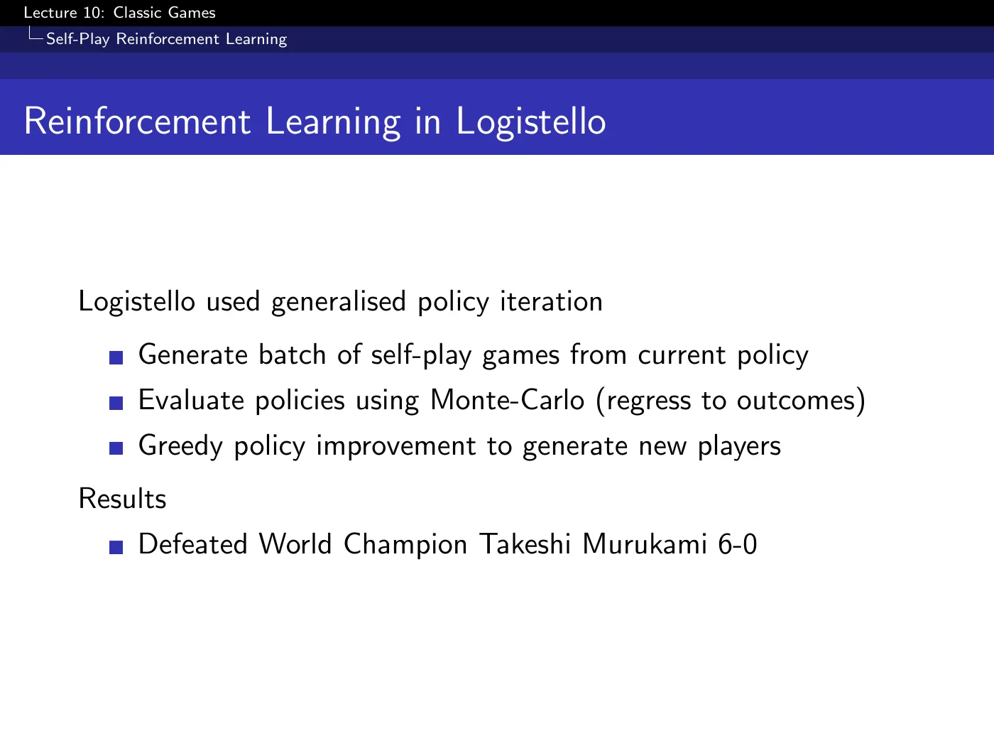
Generalized policy iteration, batched: play a few thousand self-play games, regress positions onto outcomes (Monte-Carlo evaluation), improve greedily, repeat. Result: 6–0 against the world champion, and the first superhuman program in any classic game.

The slide leaves out the ingredient that made it work

Logistello ran a full minimax search using the learned value function every time it played a move. The policy improvement step is therefore not a one-step max — it is a deep search whose leaves are the current value function.
The lecture calls this crucial. Reading p.23 as "MC evaluation plus greedy improvement" and stopping there misses why the method reached superhuman play at all.

5 · TD-Gammon

p.24–26 · Non-Linear Value Function Approximation ⏱ 52:27

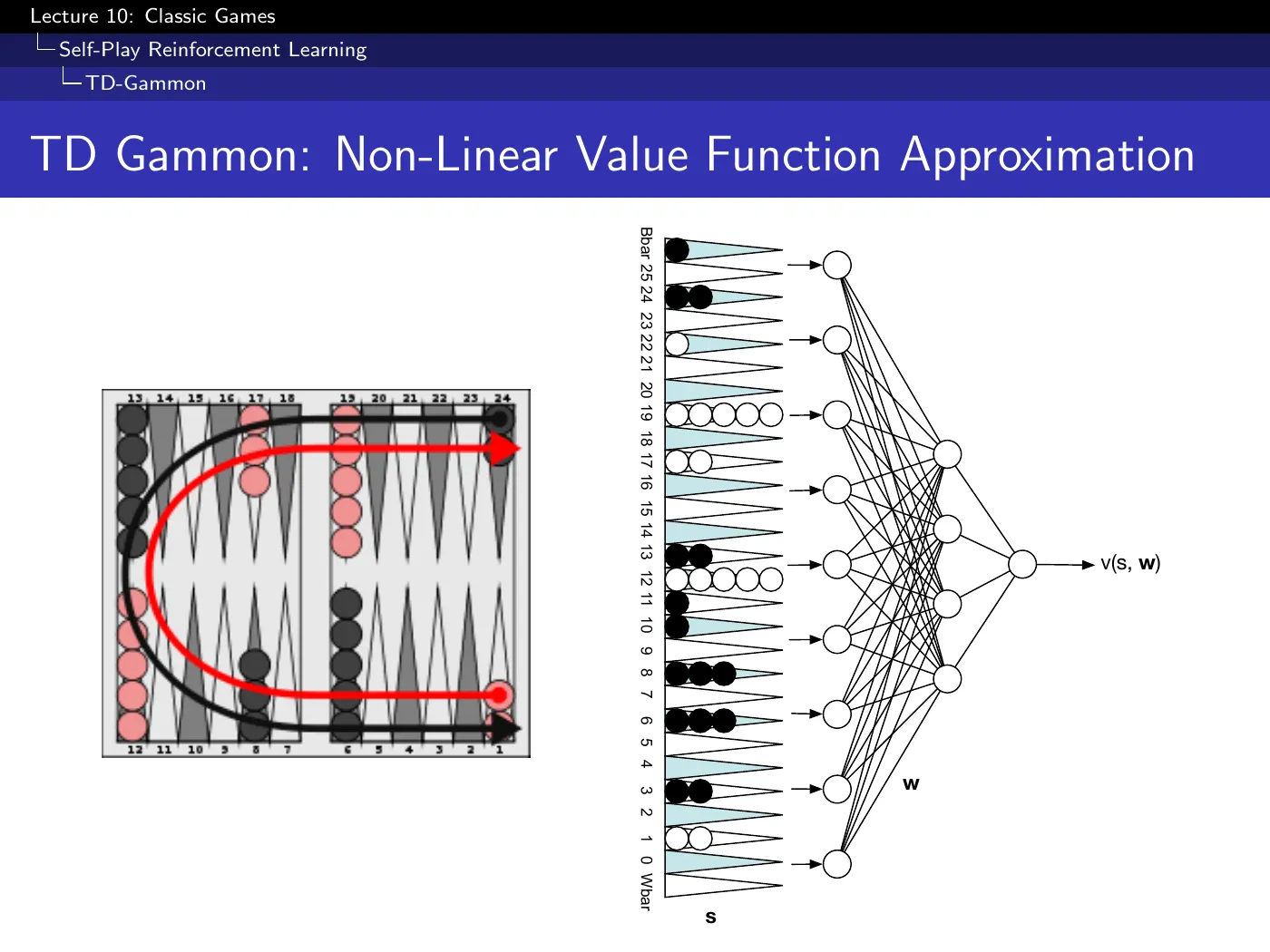
The board flattens into a binary vector with a small block of count features per location — is there one white checker here, two, three… — and that feeds a neural network with a single hidden layer of roughly 40–80 units. The only non-linear value function in the lecture's final comparison table.

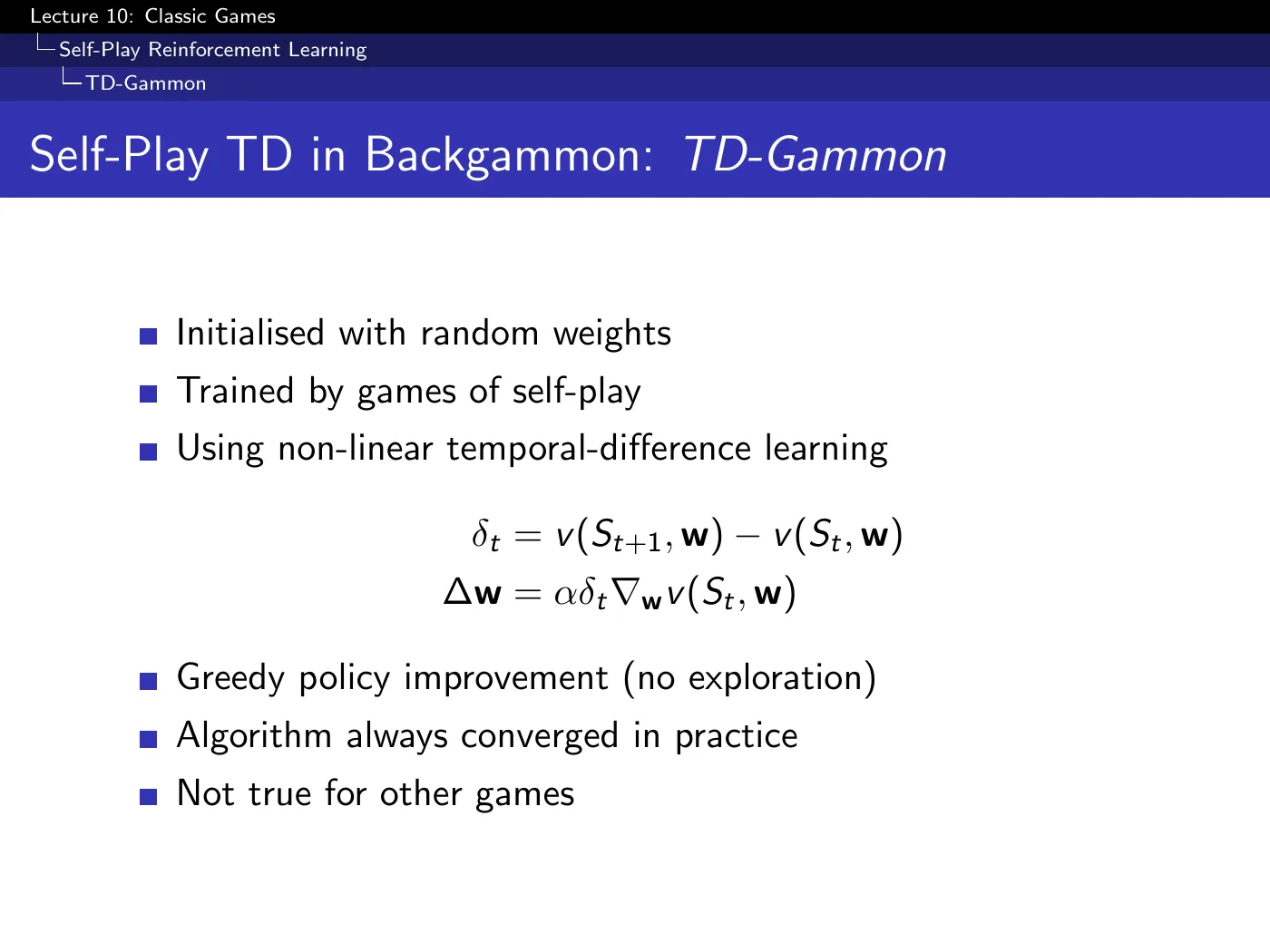
Random initial weights, pure self-play, TD( $\lambda$ ), greedy policy improvement with no explicit exploration — and it consistently converged in the reported experiments. The slide notes that the same recipe did not work reliably for other games and leaves both observations unexplained.

Both anomalies have the same one-word answer: dice

Why explicit action exploration was less necessary. Dice inject substantial state diversity even under a greedy policy. That helps coverage, but it does not mathematically guarantee that every useful action is tried.
Why the neural network may have been stable. Silver's explanation is that chance outcomes smooth the effective value landscape: a single tactical line is averaged over many possible dice rolls. Deterministic games have sharper tactical discontinuities and the same recipe often failed there.
Treat this as the lecture's domain explanation, not a convergence theorem. The algorithm still combines bootstrapping, non-linear approximation, and a changing self-play distribution — a setting that can diverge.

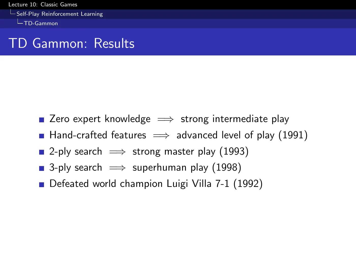
The escalation on this slide is the argument for search in miniature:

Configuration	Level
zero expert knowledge	strong intermediate
+ handcrafted features	advanced (1991)
+ 2-ply search	strong master (1993)
+ 3-ply search	superhuman (1998)

Even with the strongest value function of its era, search was still required to cross into superhuman play. Two extra ply were worth more than every handcrafted feature.

p.27 · New TD-Gammon Results ⏱ 59:18

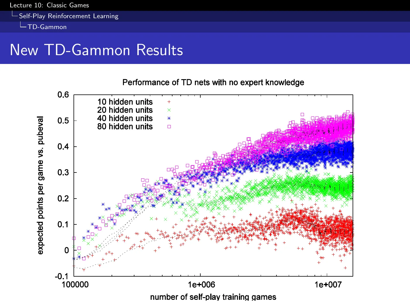
Tesauro returned around 2008 and simply trained longer on better hardware, with zero expert knowledge — raw features only. The y-axis is expected points per game against the pubeval benchmark; the x-axis is self-play training games on a log scale, out past $10^7$ ; the four series are 10, 20, 40, and 80 hidden units.

The expert features were a compute limitation, not a knowledge requirement

Trained long enough, the zero-knowledge version massively outperformed the version with handcrafted features. More hidden units are monotonically better across the whole range, and the 10-unit network actually plateaus and decays while 80 keeps climbing.
This is a 2008 result predicting the entire subsequent decade: the hand-engineering was compensating for a shortage of computation, and it stopped being necessary once the computation arrived.

Could the features the network learned be read out and taught to humans?

Not directly — but humans learned from it anyway, by watching it play. Interpreting the hidden layer is hard and largely was not done.
What happened instead is that TD-Gammon changed how humans play backgammon. Players saw openings and strategies they had not considered, adopted them, and the human standard of play rose. The knowledge transferred through behavior rather than through weights.

6 · Learning from search values

p.28–29 · Simple TD, and Where It Fails ⏱ 1:02:24

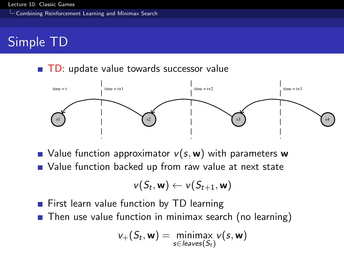
v(S_t,\mathbf{w})\leftarrow v(S_{t+1},\mathbf{w}),\qquad v_+(S_t,\mathbf{w})=\underset{s\in\text{leaves}(S_t)}{\text{minimax}}\;v(s,\mathbf{w})

Logistello and TD-Gammon both used a two-stage pipeline: learn a value function by TD, then later use it in a search. The search never improves the value function — it only consumes it at play time.

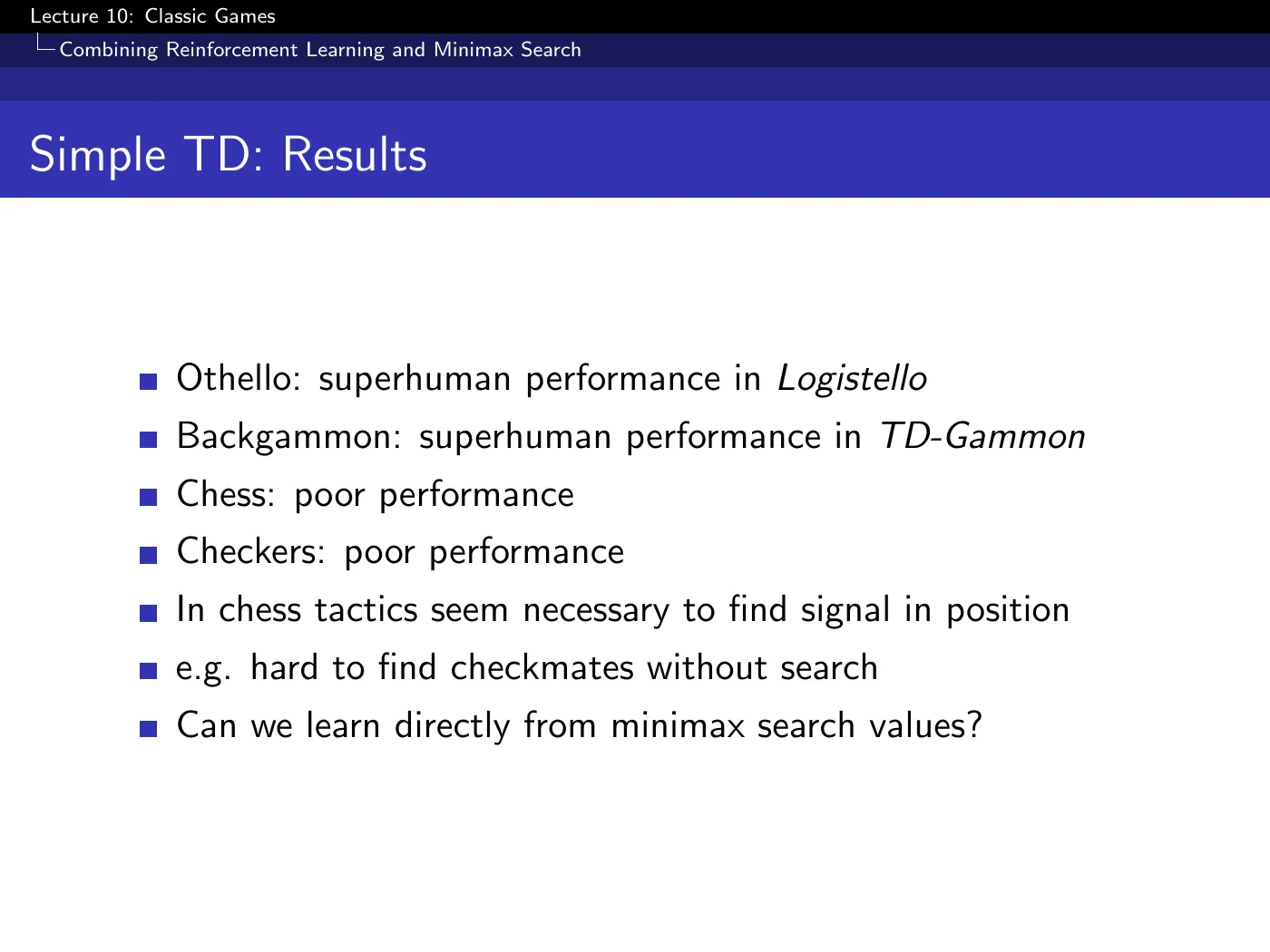
And the two-stage approach fails badly in chess and checkers.

Why tactical games break simple TD, and what that implies

A feature vector of piece counts contains no signal about checkmates, pins, or forks. Those are properties of the tree, not of the position's surface features. So a value function trained only on positions is being asked to predict something its inputs cannot see.
The fix is to get search into the learning loop, not just the playing loop — learn directly from minimax search values, so the tactical information the search discovers becomes part of what the value function is trained on.
The three algorithms that follow are three escalating answers to exactly this.

p.30–31 · TD Root ⏱ 1:05:26

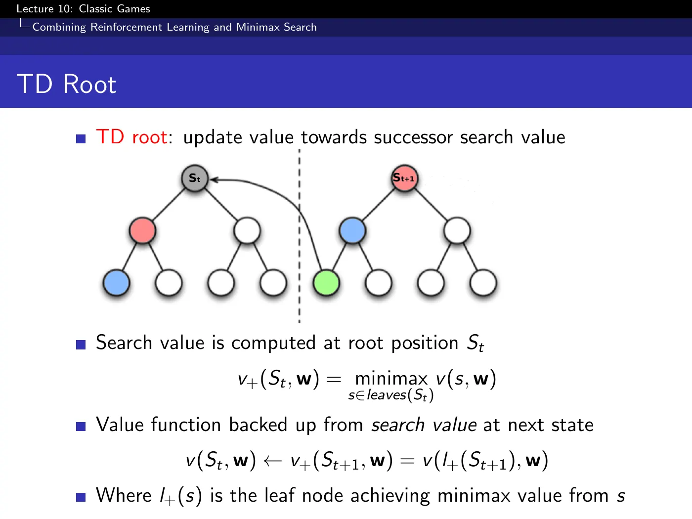
v(S_t,\mathbf{w})\leftarrow v_+(S_{t+1},\mathbf{w})=v(l_+(S_{t+1}),\mathbf{w})

Update the value function toward the search value at the next state instead of its raw value. In words: I thought black was winning; I moved, ran a deep search, and found white is winning — so I should have known that without searching.

The mechanical detail worth holding: after a tie-breaking choice, a deterministic minimax search has one selected leaf on the principal variation whose value propagates all the way to the root, so the search value is that leaf's value locally. That is why $v_+$ can be written as $v(l_+(\cdot))$ and why the displayed update touches a single leaf.

Arthur Samuel, 1959 — the first TD learning algorithm of any kind, three decades before Sutton named the family, applied to self-play checkers and beating an amateur. The slide's "other ideas we might now consider strange" is doing polite work; the good ideas were mixed with several that did not survive.

p.32–34 · TD Leaf ⏱ 1:08:33

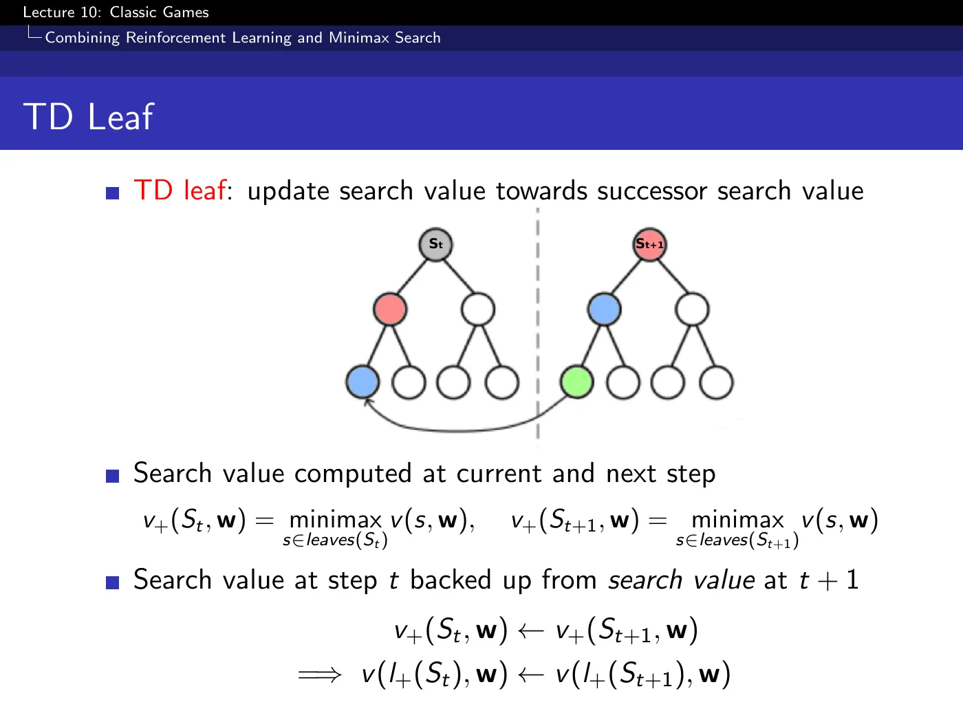
v_+(S_t,\mathbf{w})\leftarrow v_+(S_{t+1},\mathbf{w})\;\Longrightarrow\;v(l_+(S_t),\mathbf{w})\leftarrow v(l_+(S_{t+1}),\mathbf{w})

TD root improved the value function toward a search result. TD leaf improves the whole search — you want the search you run now to agree with the search you will run next step.

Why update the leaf you picked now, rather than the one the next search picked?

Away from ties, that is the only leaf that changes the current search output under a sufficiently small perturbation. The selected minimax value comes from the current principal variation; another leaf matters only after it crosses a max/min boundary and becomes principal.
A useful way to hold it: the search tree is a piecewise-linear function approximator, and the principal variation tells you which piece you are standing on. You only ever adjust the active piece. Push far enough and you cross a boundary, a different leaf becomes principal, and you start adjusting that one instead.
You do not need to remember which leaf was principal before. Only the current one matters — which is what makes this implementable.

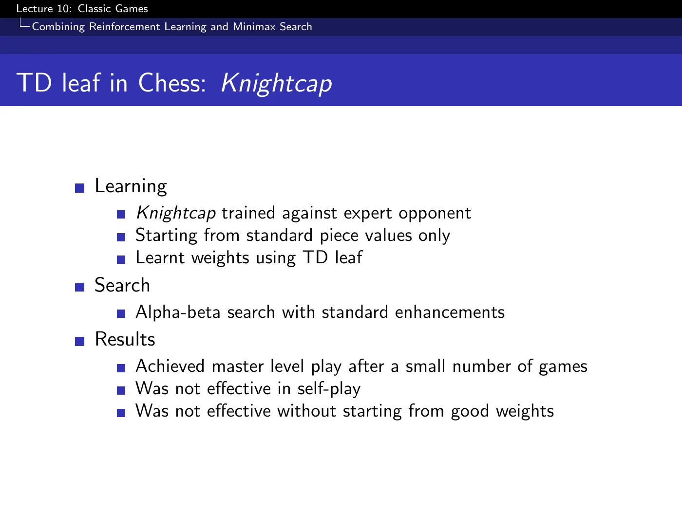
KnightCap reached master level in a small number of games — with two caveats the slide states and does not explain: it needed an expert opponent rather than self-play, and it needed sensible initial piece values rather than random weights. Both are symptoms of the same fragility, and both are what TreeStrap fixes.

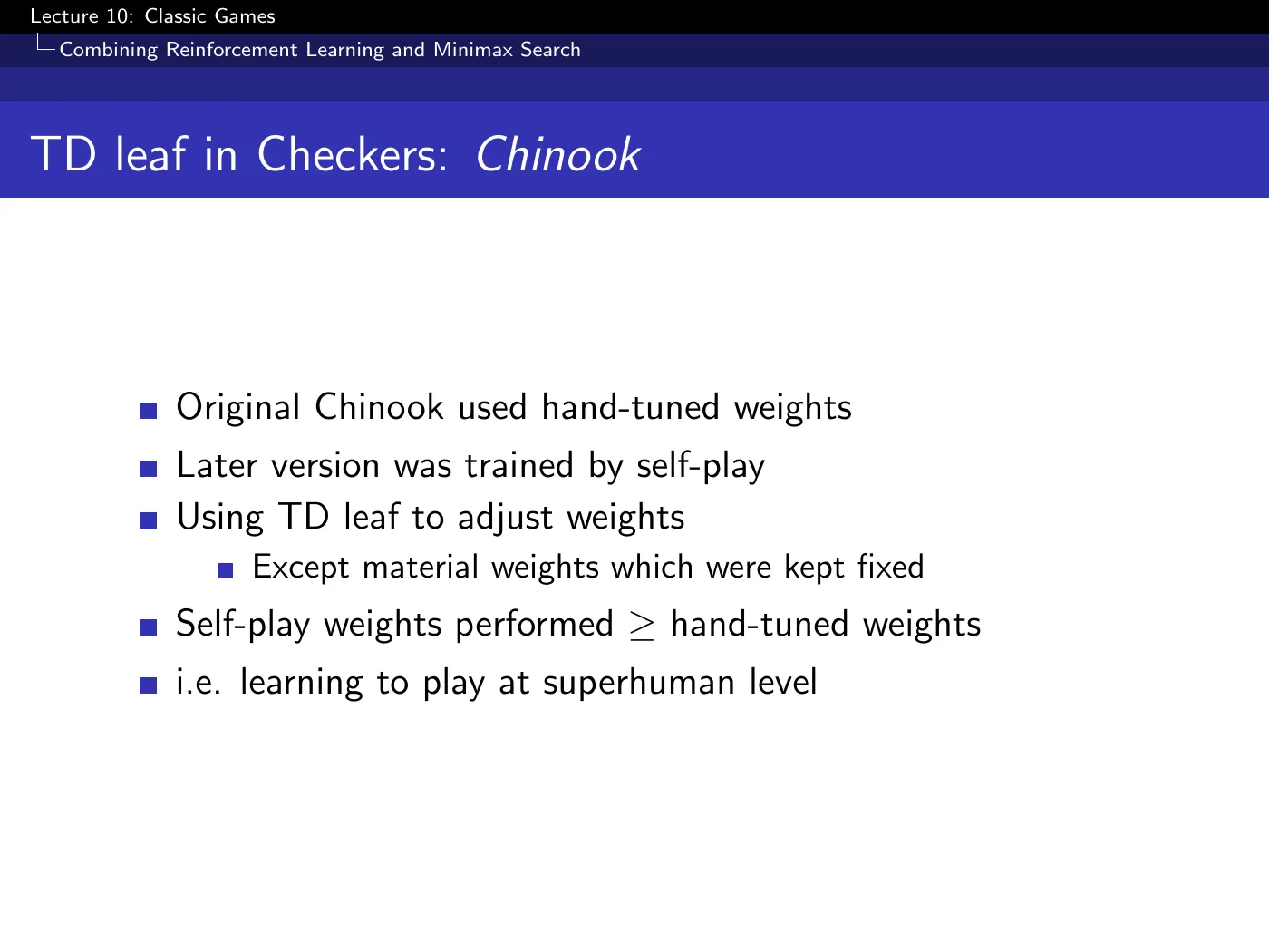
Chinook, retrofitted: TD-leaf self-play weights beat the hand-tuned ones, at a program already playing at superhuman level. Material weights were held fixed to anchor the process — a recurring pattern in these systems.

p.35–36 · TreeStrap ⏱ 1:19:55

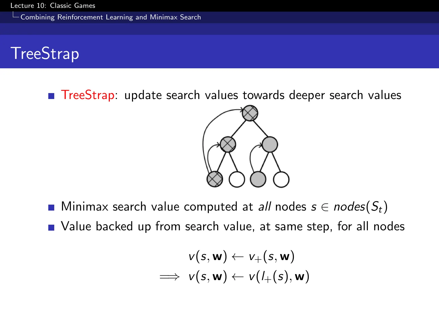
v(s,\mathbf{w})\leftarrow v_+(s,\mathbf{w})\quad\text{for all }s\in\text{nodes}(S_t)

Two changes, and each fixes one of KnightCap's caveats

Everything happens inside one search tree. TD root and TD leaf link search results across successive real positions. TreeStrap instead trains shallower node evaluations toward deeper backed-up values within the same tree. Silver presents this as the change that made self-play workable in Meep; it is an empirical design result, not a proof that mixing real and simulated backups is inherently unstable.
Every searched node becomes a training target. TD leaf uses the principal leaf from a root search; TreeStrap reuses backed-up values throughout the tree, extracting far more training signal per search. In the reported system, that richer supervision worked from random initial weights.

The unifying statement: make a shallow search predict what a deep search would have said, with the limit being a value function that predicts the deep search with no search at all.

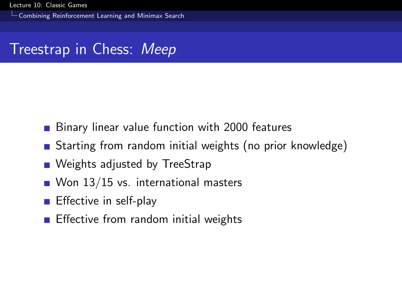
Meep: 2,000 handcrafted features, random initial weights, no piece values given, TreeStrap. It won 13 of 15 against international masters, and unlike KnightCap it worked in self-play and from random initialization.

You cannot bootstrap purely from your own search — it must be grounded

Stated as an empirical requirement and appearing on no slide: if you only ever update your value function toward your own search values, you will drift away from reality, confirming whatever you already believe with ever-deeper self-consistency.
The correction is to interleave with real game outcomes — search from positions at all stages of the game, and see enough terminal results that the tail of the value function is pinned to actual wins and losses. Every method in this section depends on it, and none of the slides say so.

7 · Simulation-based search

p.37–38 · UCT ⏱ 1:26:05

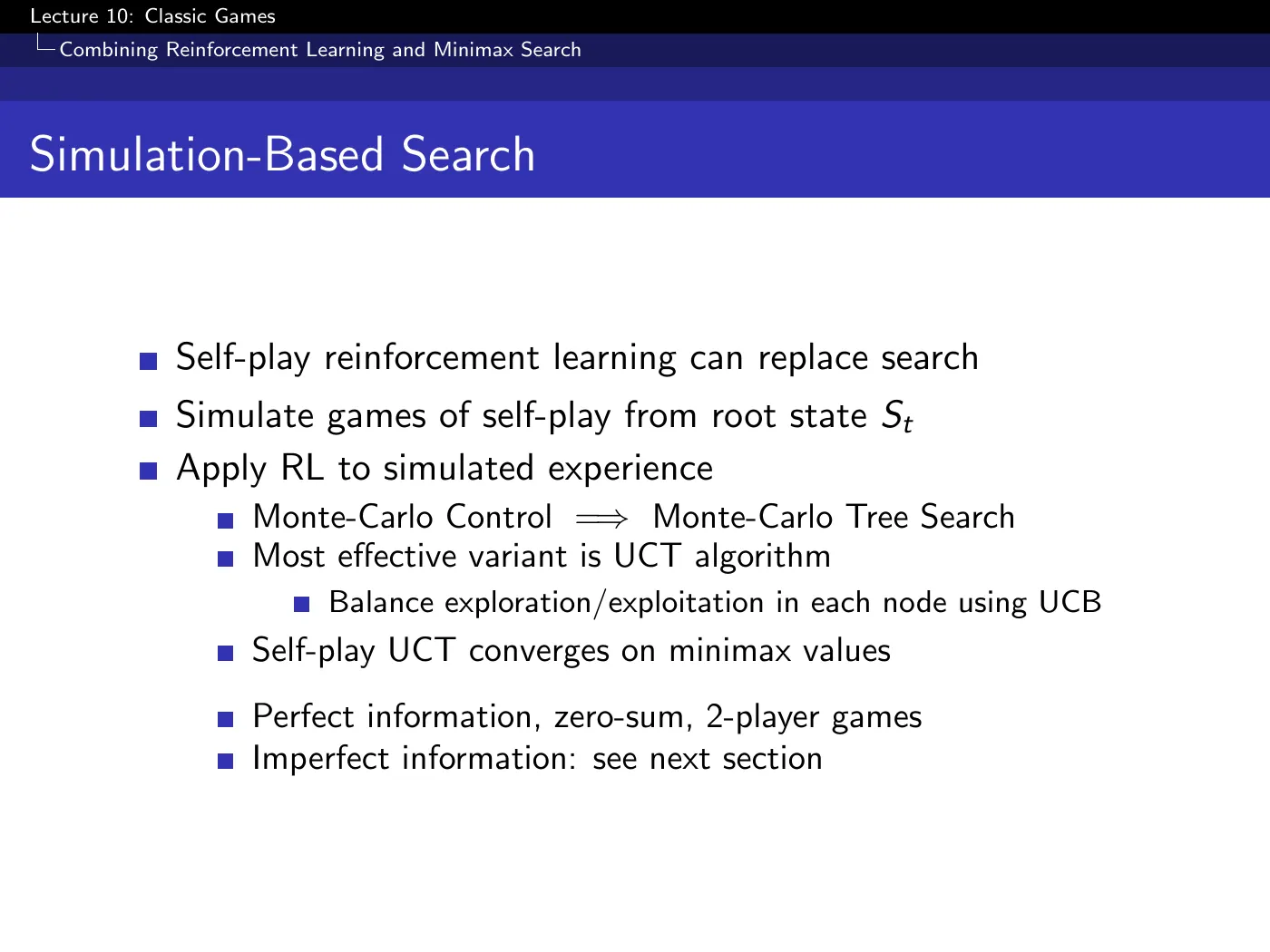
This slide finally defines UCT — the algorithm L8 and L9 both referenced without giving

UCT = MCTS where every node in the tree is treated as its own bandit problem, with an upper-confidence rule selecting the child. A common form is

A=\arg\max_a\left[Q(s,a)+c\sqrt{\frac{\log N(s)}{N(s,a)}}\right],

where $N(s)$ is the parent's visit count and $N(s,a)$ is the child-action count. This is L9's UCB idea applied locally at every tree node; the constant and exact variant depend on the implementation.
The consequence is the behavior L8 described but could not explain: most simulations flow down the principal variation, while the exploration term guarantees no branch is permanently abandoned. Systematic coverage and concentrated effort at the same time.
Under the stated finite, perfect-information, two-player zero-sum setting and persistent exploration, self-play UCT converges on the minimax values. This does not extend automatically to finite search budgets, function approximation, or imperfect information. → Lecture 8 · Integrating Learning and Planning

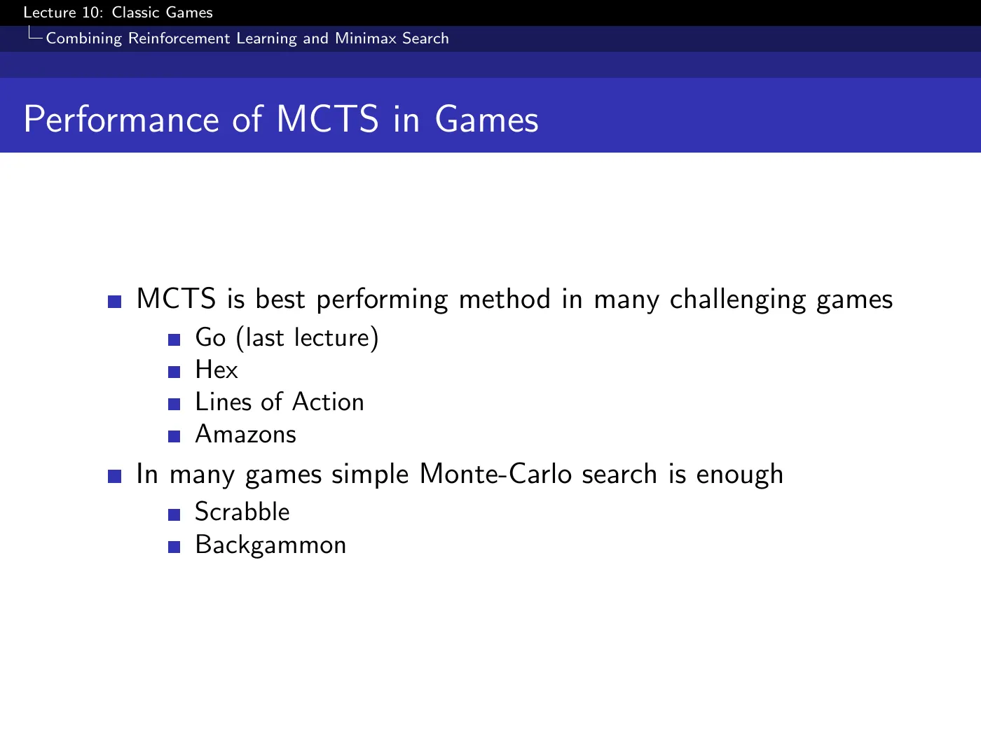
MCTS dominates where the branching factor is large or a value function is hard to build — Go, Hex, Lines of Action, Amazons. Where it is not needed, plain Monte-Carlo search suffices: Scrabble, and backgammon, where Tesauro later found rollouts beat his alpha-beta search.

p.39–40 · Maven ⏱ 1:31:23

Scrabble looks like it should be trivially solved by giving a computer the dictionary. It is not, for two reasons: top humans have memorized the dictionary — plus the anagrams and hooks — and the real difficulty is strategic rather than lexical.

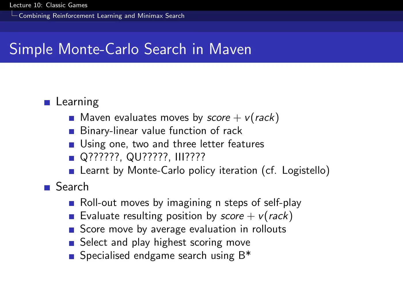
The strategy is about what you keep. Playing the highest-scoring word now can leave you with a rack that scores nothing for three turns; keeping the blank or an S sets up a 50-point bonus later. So Maven evaluates a move as immediate score + $v(\text{rack})$ , with binary features over one-, two-, and three-letter combinations left behind (Q??????, QU?????, III????) — capturing exactly that a lone Q is bad while Q with U is fine.

This is also the only game here with rewards along the way rather than a single terminal win/loss.

The search is the simplest thing that works: play the candidate word, roll out $n$ steps of imagined self-play drawing random tiles, evaluate by score plus rack value, average over rollouts, pick the best.

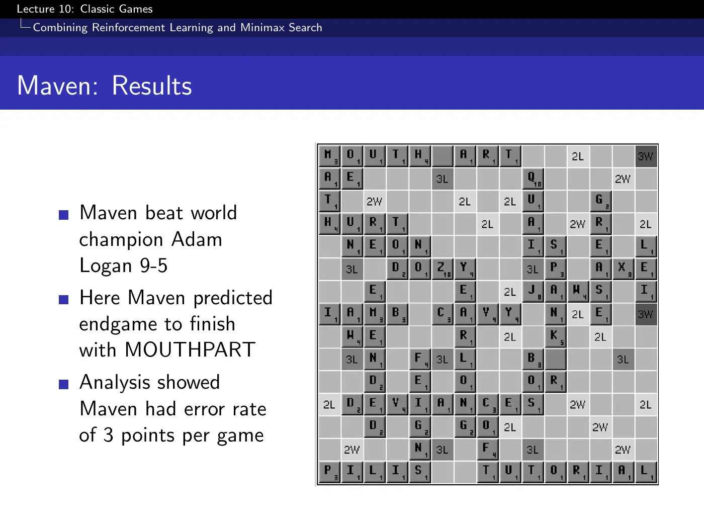
Maven beat world champion Adam Logan 9–5. The famous position: losing comfortably, Maven's rollouts found that its only winning line was to fish for one specific tile, drew it, and played MOUTHPART across two existing letters.

Rollouts capture positional consequences nobody programmed

Nothing in Maven encodes "do not open a triple word score." It does not need to: in the rollouts, the opponent actually plays on that triple word score in a large fraction of simulations, and the average score for the move drops accordingly.
Simulation converts a strategic principle into an empirical measurement. That is the general reason search substitutes for knowledge.

The lecture disputes its own slide here

The slide reports Maven playing within 3 points per game of perfect. Silver's verdict on that figure: "I suspect this result is bogus."
The analysis assumed naive rollouts are optimal, but a proper MCTS that models the opponent's replies and the contingencies after them would likely play better still. Treat 3 points per game as "close to what humans believed optimal in 2002", not as a bound.

8 · Imperfect information

p.41–43 · Smooth UCT ⏱ 1:40:29

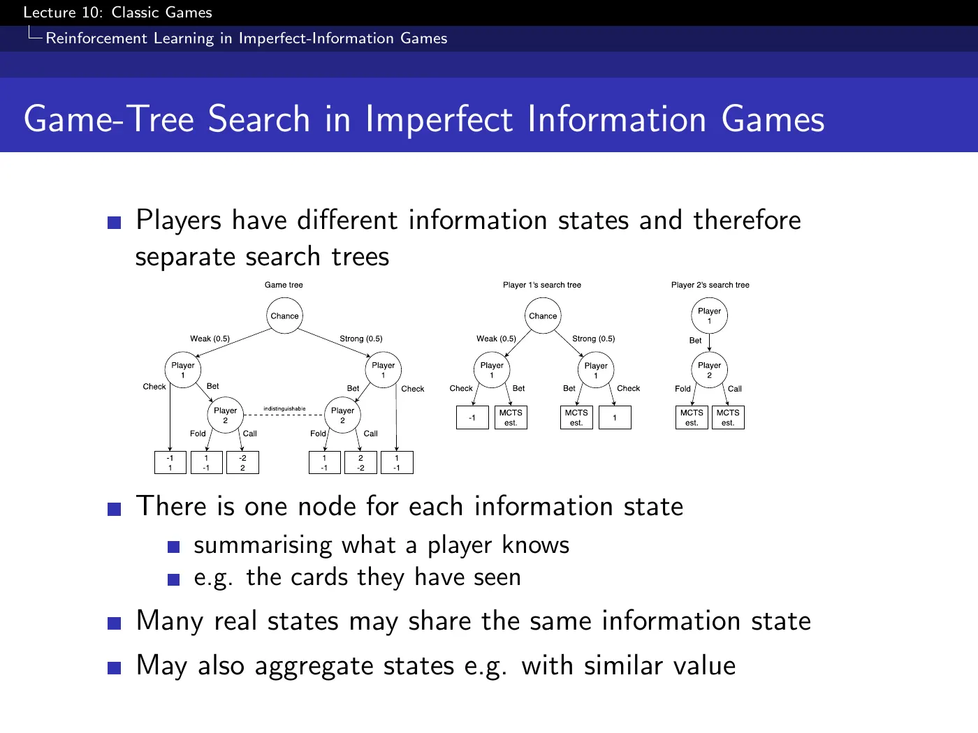
With hidden information, players know different things, so each player needs their own search tree, with one node per information state rather than per real state. Many real states collapse into a single information state — every deal consistent with what you have seen.

The players' trees are coupled: each picks actions from its own tree, but the resulting simulations update statistics in the others'.

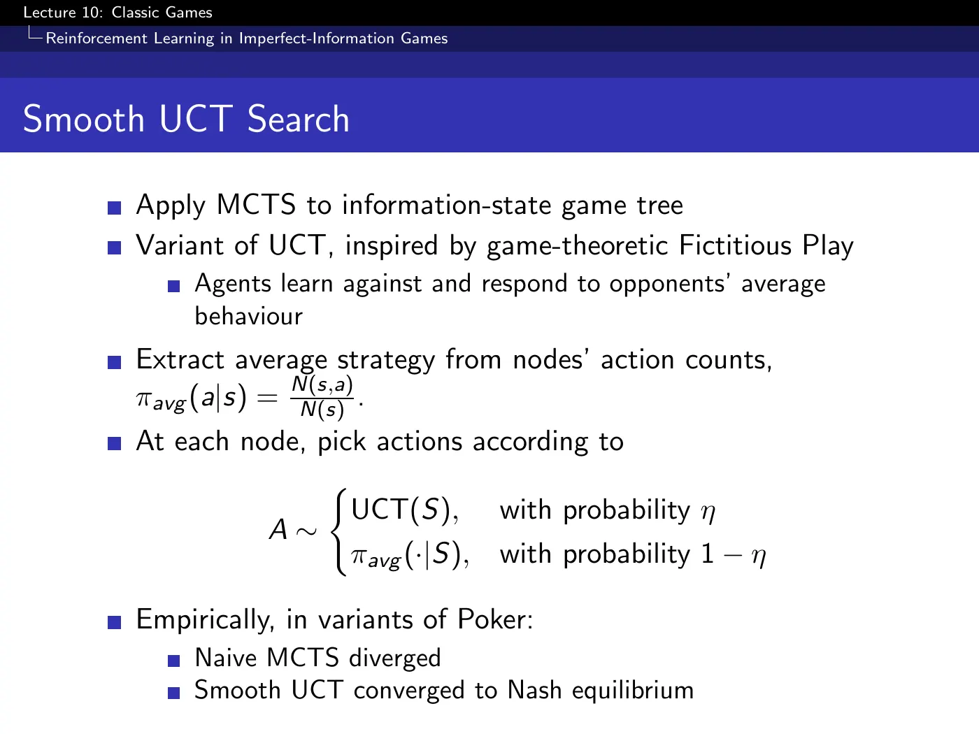
\pi_{\text{avg}}(a|s)=\frac{N(s,a)}{N(s)}, \qquad A\sim\begin{cases}\text{UCT}(S) & \text{w.p. }\eta\\ \pi_{\text{avg}}(\cdot|S) & \text{w.p. }1-\eta\end{cases}

Naive MCTS diverges here — this is not a small adaptation

Take UCT, the method that works well in Go, apply it to poker, and it fails. It does not reach a Nash equilibrium.
The fix comes from fictitious play: respond to the opponent's average historical behavior, not their current behavior. The average strategy is free — it is just the action counts already stored at each node, normalized.
Mixing a fraction of average-strategy play into UCT stabilized the studied poker variants. The reported result is empirical: Smooth UCT approached Nash behavior where naive MCTS did not. Do not read it as a general convergence theorem for all imperfect-information games.

The result that should be surprising

Around the same time, a University of Alberta program essentially solved heads-up limit Hold'em — so close to Nash that distinguishing it from equilibrium play would take about a million years of hands.
SmooCT outperformed it at the computer poker competition — while losing to it head-to-head. Nash equilibrium is a guarantee of not being exploited, not a promise of exploiting others. Against a varied field, an agent that has practised the situations that actually arise between learning opponents wins more, because self-play concentrates its experience on exactly those positions.
A perfect defensive strategy and the best tournament strategy are different objects.

9 · The recipe, and the assumption that broke

p.44 · RL in Games: A Successful Recipe ⏱ 1:46:37

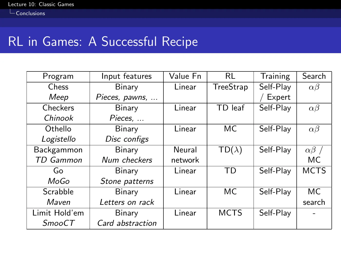
The summary table, read column-wise, shows a strong historical pattern: binary features → often a linear value function → self-play → some form of search.

Several learning rules can be viewed through the return-versus-bootstrap spectrum: MC is the $\lambda=1$ endpoint, TD uses bootstrapping, and TD-leaf or TreeStrap use search-backed targets. They are related, but TreeStrap and MCTS are not literally just ordinary TD( $\lambda$ ) with a different $\lambda$ .

The lecture closes by contradicting itself, months before the world found out why

Silver had argued for years — in papers, and for most of this lecture — that Go requires search, because no function approximator could be expressive enough to capture that game's nuance from a position alone.
Then, in the final three minutes: "we just did that a few months ago" — a very deep neural network that plays Go well just by reading out the network, alongside an MCTS with a million simulations.
That is AlphaGo, described in passing in a 2015 lecture, before the Nature paper. Read the last slide's "mostly linear" column against it: this table was about to acquire a very different row.

Search and knowledge are the same currency

The closing idea, on no slide: there is a trade-off between search and knowledge. You can put understanding into the value function by learning, or you can acquire it at run time by searching deeper. There are two ways to improve — search deeper, or learn better — and they are flip sides of one coin.
That is the sentence to carry out of the whole course. Deep Blue bought its strength almost entirely with search; TD-Gammon bought most of its with learning; AlphaGo bought a great deal more with learning and still kept the search.

Study checklist

Close the note and answer these in your own words. Reopen only the section linked after the question.

What recurring roles do self-play, a value function, and search play in the case studies? → The one idea
What is unique in a two-player zero-sum game: the minimax value, the policy, or both? → 2 · Game theory, minimally
Why does a fixed point of mutual best responses form a Nash equilibrium, and why need self-play not reach one? → p.6–7 · Best Response and Nash Equilibrium ⏱ 7:41
Under $\pm1$ terminal rewards, how is value related to win probability? → p.10–11 · The Minimax Value Function ⏱ 21:23
Why does truncated minimax search need a value function at its leaves? → 3 · Minimax search
What terminal boundary condition is omitted by the reward-free interior TD update on p.20? → p.20–21 · Self-Play TD and Afterstates ⏱ 42:38
Under what condition can afterstate values replace $Q(s,a)$ ? → p.20–21 · Self-Play TD and Afterstates ⏱ 42:38
Why should the “dice explain TD-Gammon” story be treated as an empirical hypothesis rather than a guarantee? → 5 · TD-Gammon
How do TD root, TD leaf, and TreeStrap bring search values into learning at different places? → 6 · Learning from search values
Define UCT and state the assumptions behind its minimax convergence claim. → 7 · Simulation-based search
Why can naive MCTS fail in imperfect-information games, and what does Smooth UCT mix in? → 8 · Imperfect information
Explain the search-versus-knowledge trade-off using two systems from the lecture. → 9 · The recipe, and the assumption that broke

Gaps to close on your own

No slide in this deck is skipped — the lecture covers all 44 pages. What follows is named-but-not-developed material.

Alpha-beta search is never explained. It appears in the recipe table for four of the seven systems and is explicitly set aside: "what I'm not going to talk about today is how to make this efficient." Decades of research sit behind that entry — it prunes branches that provably cannot affect the minimax value. If you intend to build anything in this space, this is the largest single gap in the lecture.
AlphaGo. Described in three minutes at the end, before publication. The paper is Silver et al., Mastering the game of Go with deep neural networks and tree search, Nature 2016 — and it is the direct continuation of this lecture: exactly the recipe on p.44 with a deep network in the value-function column, plus a policy network, plus MCTS.
Convergence, summarized. Exact minimax search returns minimax values when it reaches terminal states; suitable tabular minimax-RL algorithms and self-play UCT have convergence results under their stated assumptions. Every practical system in this lecture adds approximation, finite search, or other details outside those simple statements, and TD-Gammon in particular used a combination known to be able to diverge. The gap between what is proved and what works is unusually wide here.
Card abstraction in poker. SmooCT's input features are listed as "card abstraction" and never described. Grouping strategically similar hands is what makes the information-state tree tractable at all.
Counterfactual regret minimization. Named on p.42 as the method that achieved "perfect" play in heads-up limit Hold'em, and not explained. It is the dominant approach in imperfect-information games and the natural counterpart to everything in section 8.
Retrograde analysis and endgame databases. Chinook's backward search is described in one line. The construction — enumerate all positions with $\le n$ pieces, solve them exactly backwards from terminal states — is what allowed checkers to be solved outright in 2007.
Maven's opponent modeling. Maven samples the opponent's rack uniformly from remaining tiles, which ignores that opponents reveal information by how they play. Silver flags this as naive and notes later programs exploit it; no method is given.

Language notes

Phrasings worth stealing for your own technical writing and talks:

Expression	Use
the Drosophila of artificial intelligence	a simple domain adopted as the field's standard testbed
microcosms encapsulating real world issues	a toy problem that preserves the difficulty that matters
a meaningful IQ test	a benchmark with an external, credible standard
plays perfectly against God	provably optimal, not merely unbeaten
it needs to get off the ground first	a method requiring a decent initialization to work at all
you have to ground it	tie a self-referential process to external evidence
you can end up kidding yourself	a self-confirming loop that drifts from reality
I suspect this result is bogus	doubting a published figure, plainly and with a reason
we should always question our assumptions	prefacing the retraction of your own prior claim
flip sides of the same coin	two apparently distinct routes that trade off against each other