Silver RL·Lecture 2·Lecture Notes
Lecture 2 · Markov Decision Processes
Slides: David Silver, UCL Course on Reinforcement Learning (2015), CC BY-NC 4.0. Some slide content is from third parties and is outside that licence.
Slides: David Silver - RL Course (UCL 2015) · Previous: Introduction to RL (L1) · Next: Lecture 3 · Planning by Dynamic Programming
Companion: Silver RL Lecture 2 — Question List (your own stuck points, in Korean) · Markov Decision Process (MDP)
Read this instead of watching. Each slide is embedded below with only what the slide itself does not say — the reasoning, the caveats, and the questions worth being able to answer.
The one idea
L2 builds the MDP by adding one ingredient at a time, and each addition creates exactly one new question:
| Object | Tuple | New ingredient | New question |
|---|---|---|---|
| Markov process | — | what happens? | |
| Markov reward process | reward | how good is it? | |
| Markov decision process | actions | what should I do? |
Each layer inherits everything below it, so once you can evaluate an MRP you can evaluate any MDP with a fixed policy — because fixing a policy collapses an MDP back into an MRP (p.27).
Both say value now = immediate reward + discounted value of where you land. They differ in one symbol:
Expectation → evaluation (how good is this policy). Optimality → control (how good is the best policy).
The consequence is immediate and decides everything downstream: the expectation equation is linear and can be solved by matrix inversion; the optimality equation contains a , is non-linear, and has no closed form. That single fact is why L3 exists.
Not . Knowing tells you how much reward is available but not how to get it — you would still need a one-step lookahead through and to choose.
Knowing finishes the job: , no model required. Hold onto this, because L5 spends its first ten minutes rediscovering it as the reason model-free control uses rather than .
Contents
- 1 · The Markov property
- 2 · Markov reward processes
- 3 · The Bellman equation for MRPs
- 4 · Adding actions
- 5 · Value functions and the Bellman expectation equation
- 6 · Optimality
- 7 · The Bellman optimality equation
- Study checklist
- Gaps to close on your own
- Language notes
1 · The Markov property
p.3–6 · Markov Property and Markov Processes ⏱ 3:05
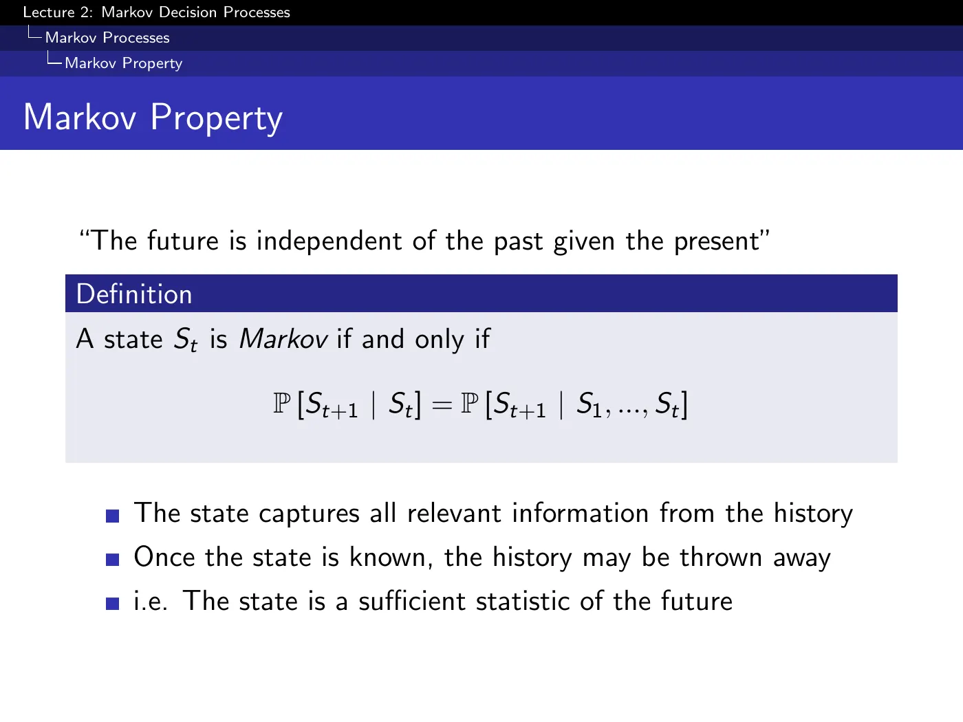
"The future is independent of the past given the present." The operational phrasing is better: the state is a sufficient statistic of the future, so once you know you may throw the history away.
The slide claims almost all RL problems can be formalized as MDPs, and the three examples are each doing work:
- Optimal control is a continuous MDP — the differential-dynamics framing is the same object with continuous and .
- Partially observable problems are not exceptions; they convert into MDPs (p.53 shows how).
- Bandits are MDPs with one state. Which is why L9 can spend an hour on bandits and call it reinforcement learning.
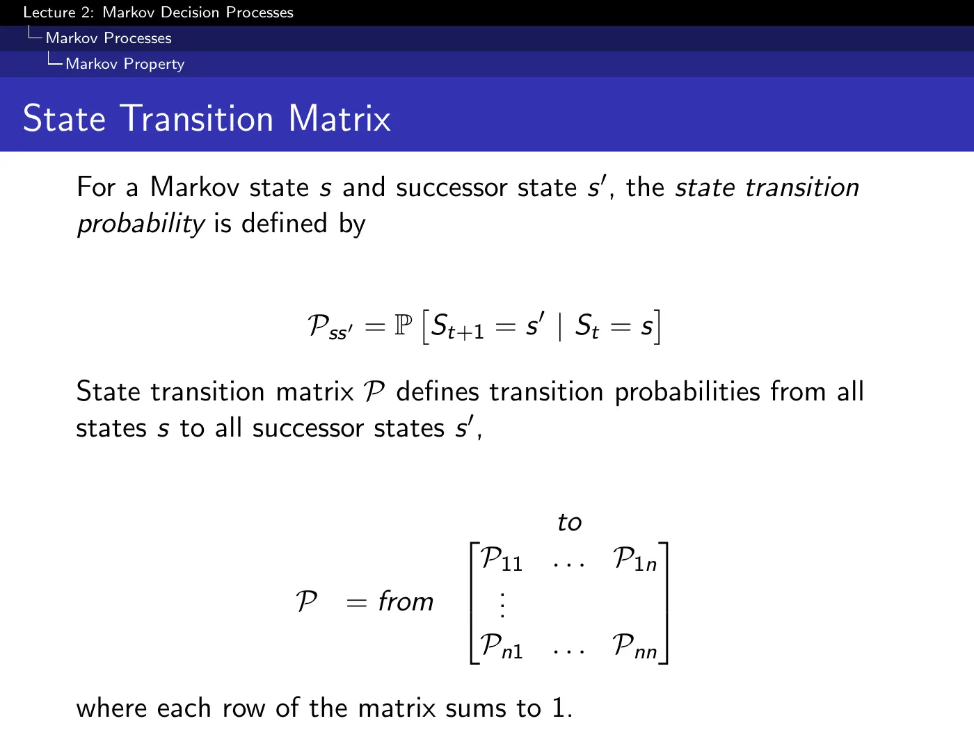
has one row per state, each summing to 1. That single matrix is the entire dynamics.
Two answers, and the second is the more useful one.
(1) Allow non-stationarity and use the same algorithms, incrementally tracking the drifting solution rather than converging to a fixed one. This is exactly the constant- argument in L4.
(2) Absorb it into the state. If the probability depends on how long you have been somewhere, then how long you have been there is part of the state. Add a counter and the process is Markov again — at the cost of many more states, possibly infinitely many.
Option 2 is the deeper point: "non-Markov" usually means "your state is missing something." The small diagrams in this lecture are chosen to fit on a page; MDPs routinely have states.
p.7–9 · Student Markov Chain ⏱ 7:44
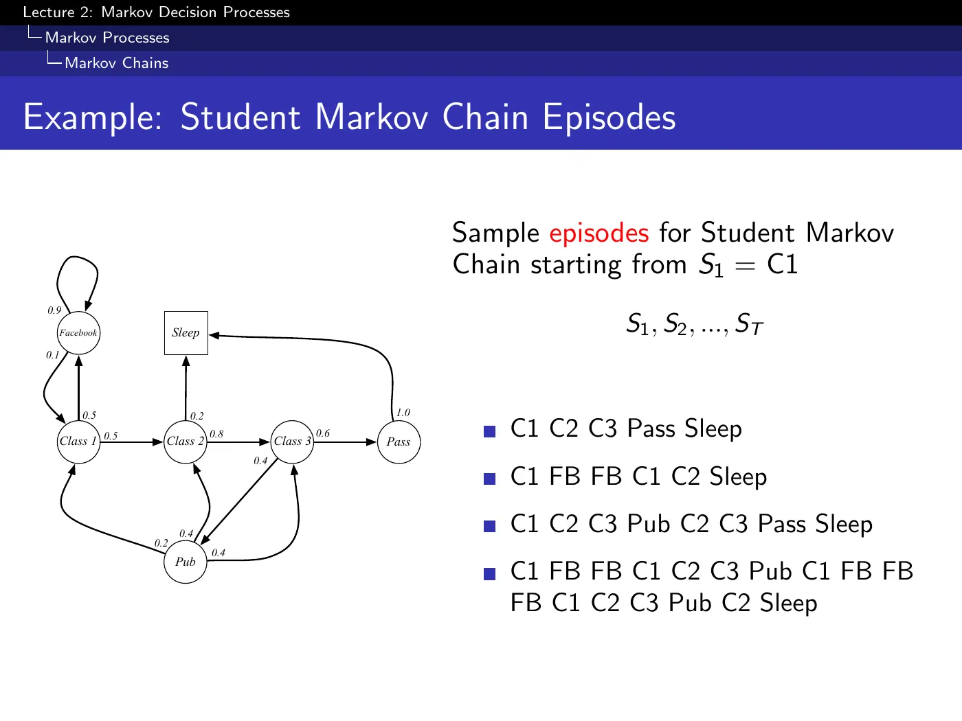
Three classes, Facebook as a distraction with a self-loop, a pub, and Sleep as a terminal state.
A terminal state needs no special machinery — it is just an absorbing state with a self-loop of probability 1 collecting zero reward forever. Worth knowing early, because it means "episodic" and "continuing" are not two different formalisms.
The samples are variable-length sequences drawn from the chain. There is no reward yet and nothing to decide; this is only what happens.
2 · Markov reward processes
p.10–13 · Reward, Return, and Discounting ⏱ 13:04
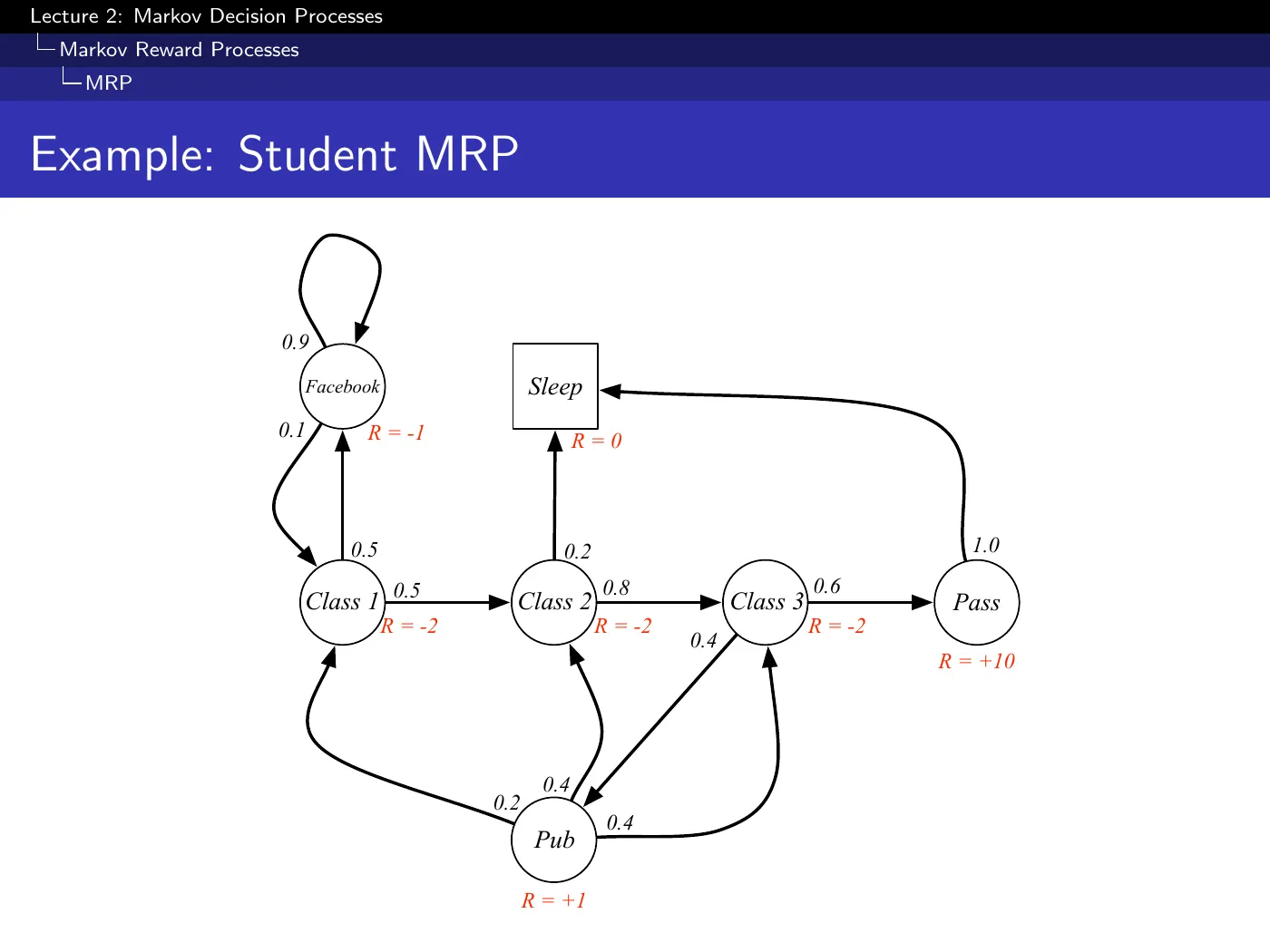
Two things to keep straight from the start:
- is immediate reward — one step only.
- is a random variable, one sample of a whole trajectory. There is no expectation in it yet. That arrives with the value function two slides later, and the distinction is the source of most early confusion.
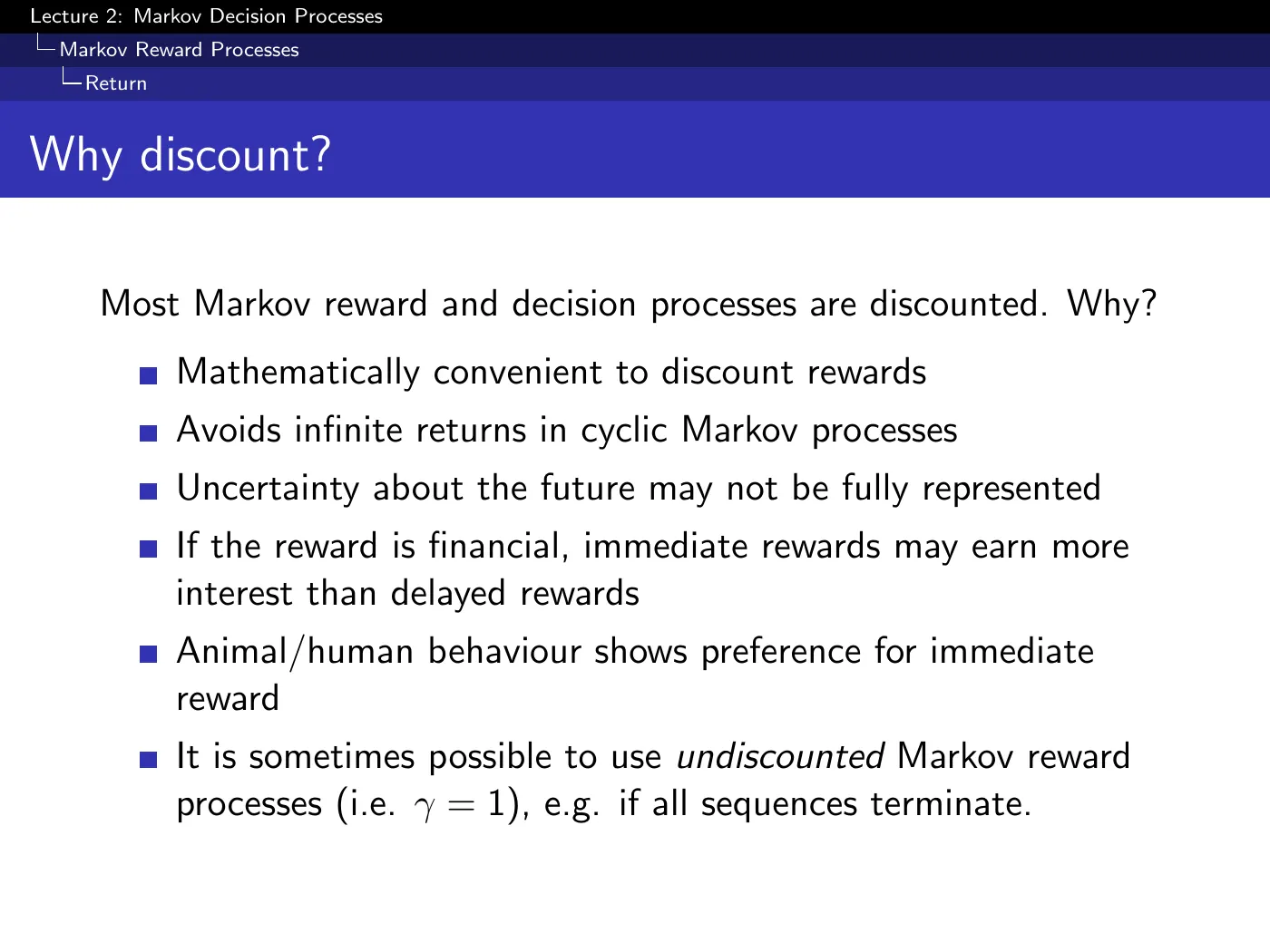
The slide lists six. In the lecture the ordering is explicit and worth inheriting:
- It is mathematically convenient — stated as the main reason, plainly.
- It bounds returns in cyclic processes. Without it, a loop that keeps collecting reward gives and the mathematics stops working.
- It represents an imperfect model. This is the intuitive one: a plan promising a bigger reward in ten years requires you to trust your model for ten years. Discounting is how much you trust it.
- Interest rates, if reward is money — behaves like the inverse of an interest rate.
- Humans and animals genuinely prefer immediate reward (roughly hyperbolic, not exponential).
And the escape hatch: if all sequences terminate, is fine.
No — any single drawn sample terminates, provided no state has a self-loop of probability exactly 1 that traps you. The process contains infinite loops; each sample is finite, and only its length is random.
The exception matters: a probability-1 self-loop does produce an infinite sample. That is precisely when you need , or the technical conditions, or the average-reward formulation on p.54–56.
p.14–18 · The Value Function ⏱ 23:04
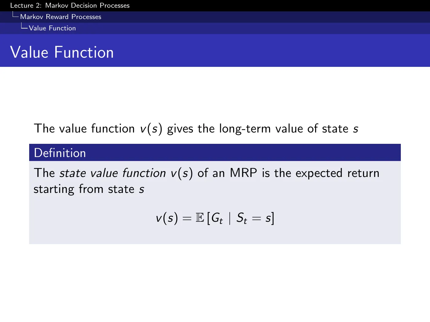
The returns are random; the value function is not. is an expectation over trajectories — a fixed number attached to a state. Holding that apart from is what makes the next hour parse.
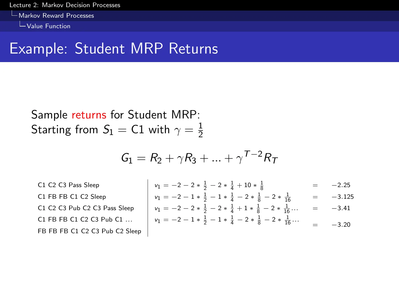
The four sample returns from at give — all different, all legitimate samples of the same quantity. Averaging enough of them estimates , which is exactly Monte-Carlo evaluation in L4, arriving three lectures early without being named.
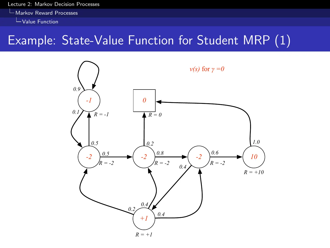
At the value of every state is just its own immediate reward: , because nothing beyond one step is visible. The for passing is worth nothing from two states away.
At , rises to about — the same state, revalued because the eventual now reaches back through the chain.
is not a nuisance parameter. It defines what problem you are solving, and the same MDP with different has genuinely different optimal behavior.
3 · The Bellman equation for MRPs
p.19–21 · The Decomposition ⏱ 29:52
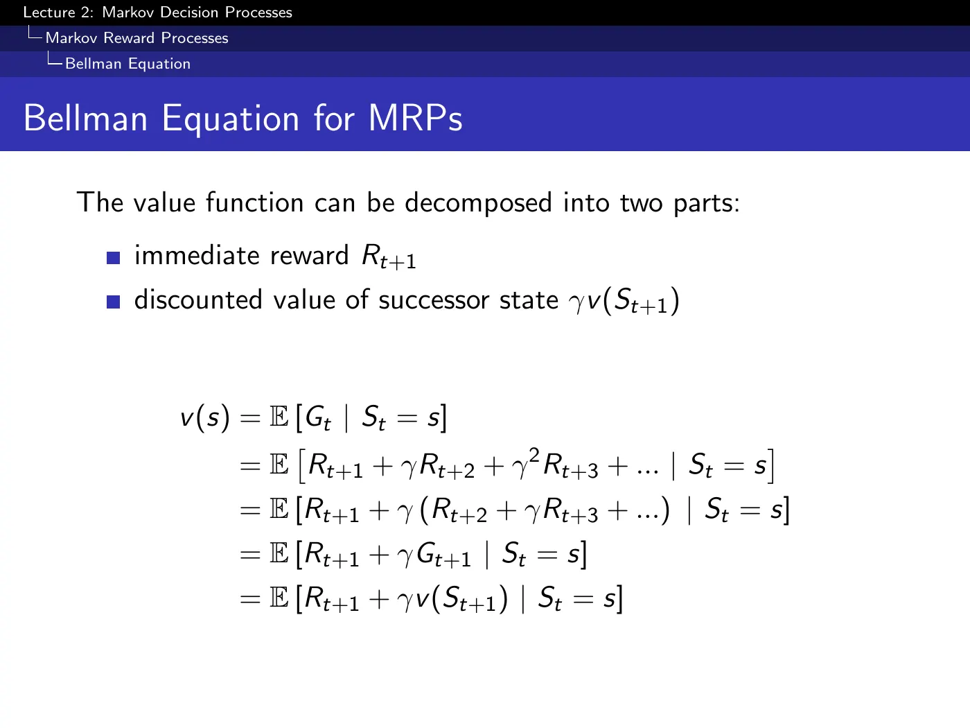
The derivation is four lines and each has a name worth knowing: unroll ; factor out ; recognize the remainder as ; then apply the law of iterated expectations to replace with .
That last step is the only non-mechanical one — it is what turns a statement about trajectories into a statement about states.
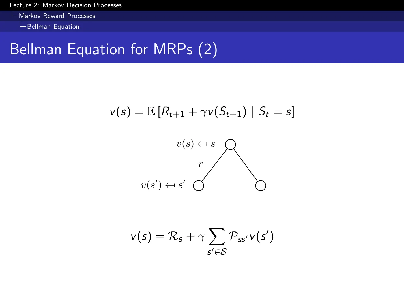
It does not compute ; it characterizes it. If your numbers satisfy it everywhere, they are the value function. If they do not, they are not.
That is why p.21 verifies rather than derives: checks one state's self-consistency. Every algorithm in L3–L8 is a way of forcing this equation to hold.
The convention follows Sutton & Barto: the agent acts, control passes to the environment, and everything that comes back carries the new time index. So the reward for leaving state is .
Nothing mathematical depends on it — re-index throughout and every result is unchanged. The lecture notes its own slides may be inconsistent on this point. Read the diagrams as you exit a state, you collect its reward, and do not let the subscript mislead you.
p.22–23 · Matrix Form and Direct Solution ⏱ 38:41
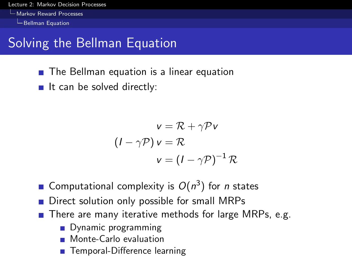
Because the Bellman expectation equation is linear, an MRP can be solved exactly, in one shot. No iteration, no learning, no approximation.
Then the bill: for states. That kills it for anything real, and the slide names its three replacements in order — dynamic programming (L3), Monte-Carlo (L4), TD learning (L4).
Everything from here to L10 is a response to this one complexity bound. When the same reappears in L6 for LSTD and in L8 for solving a learned model, it is this same inversion.
Note also what linearity depended on: averaging over a fixed policy. Once you introduce a (p.48), linearity is gone and so is the closed form.
4 · Adding actions
p.24–25 · The MDP ⏱ 43:19
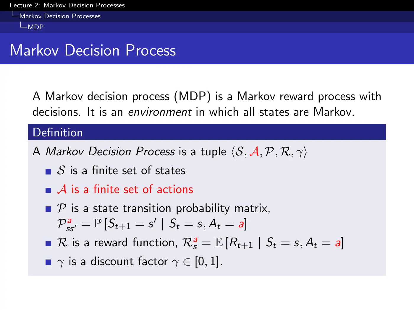
. Both and now carry a superscript — think of one transition matrix per action.
The reward depending on the action is not a technicality. A trading agent that buys £1,000 of goods pays £1,000 for the action, regardless of where it lands. Costs attach to what you do, not only to where you end up.
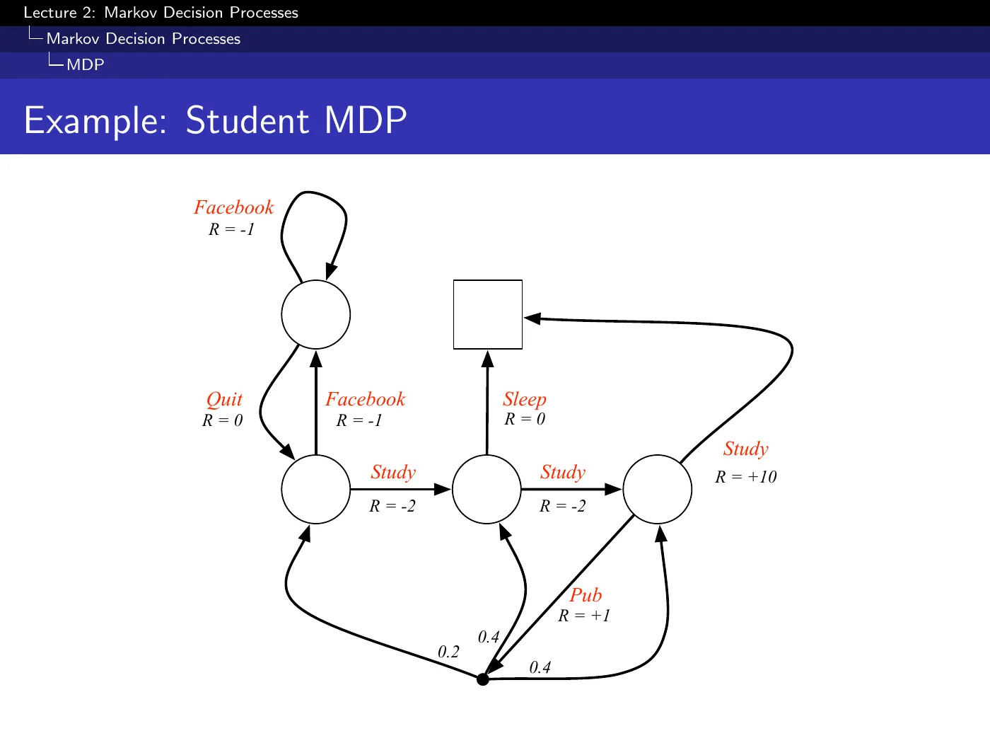
Pub was a state; it is now an action. The diagram gained black dots (action nodes) between the white circles (states), and that is where the environment's randomness now lives: you choose Pub, then the dice decide whether you land in , , or .
Every other action also has a black dot, with transition probability 1 — they are simply not drawn. Reading the diagram as "some arcs are stochastic and others are not" misses that all of them pass through the same two-stage structure: your choice, then the environment's roll.
p.26–27 · Policies ⏱ 46:23
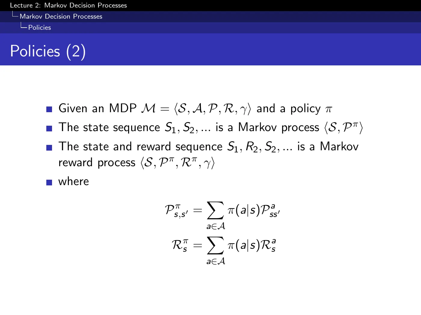
Policies are stationary — they depend on the state, not on . That is not a restriction but a consequence: the Markov property says already contains everything relevant, so a time index would add nothing.
Average the dynamics over your own action choices and the actions vanish — the state sequence is a Markov process, the state-and-reward sequence a Markov reward process.
This is the structural reason prediction and control are separate problems, and why every prediction method in the course is really an MRP method. L4's driving-home example is stated as an MRP for exactly this reason.
Because the state already characterizes all future reward. The Markov property guarantees is a sufficient statistic, so a policy conditioning on has everything it needs.
The sharper point: past rewards are irrelevant to optimal behavior. Already banked a million, or lost one? Neither changes what is best to do now. Optimality always looks forward from the current state, which is what makes a state-conditioned policy sufficient rather than merely convenient.
5 · Value functions and the Bellman expectation equation
p.28–29 · Two Value Functions ⏱ 51:01
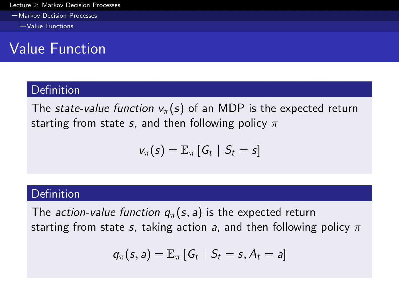
The subscript is new and necessary: with actions there is no longer one expectation. Different policies induce different distributions over trajectories, so "how good is this state" is ill-posed until you say under what behavior.
is the one that will matter. It is the quantity you compare when choosing — "should I go left or right" is answered by comparing values, not values.
p.30–35 · The Backup Diagrams ⏱ 54:51
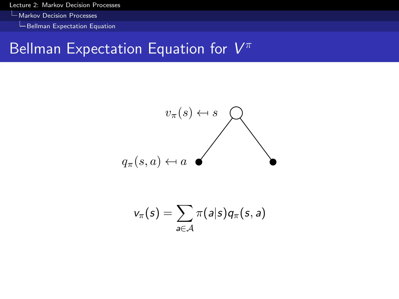
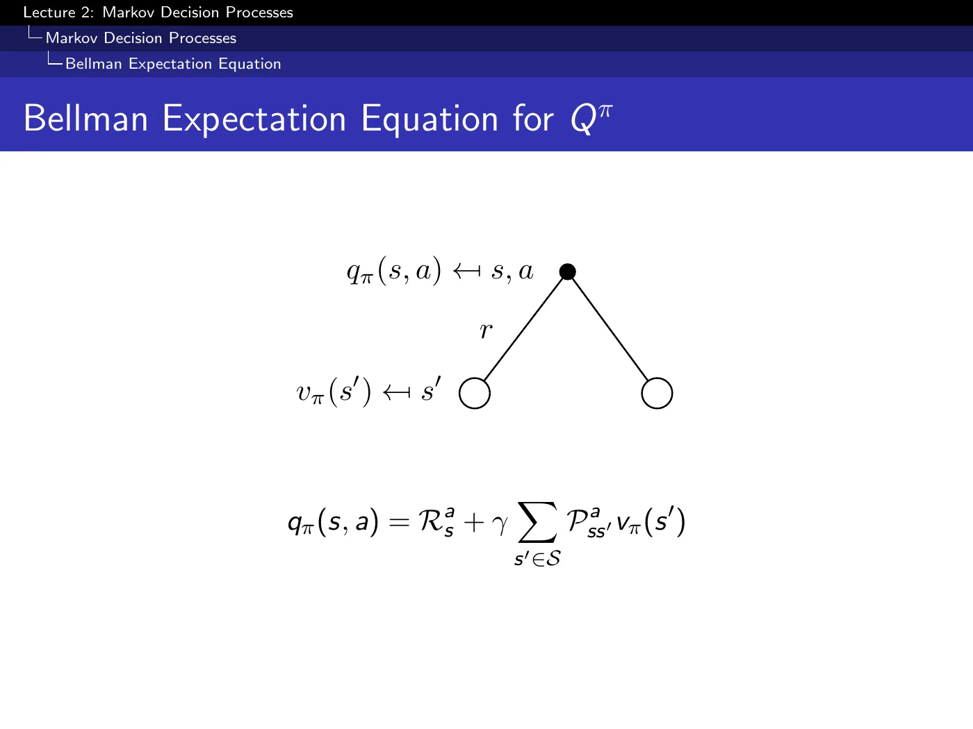
(white node down to black): average over your policy. You control this.
(black node down to white): average over the environment's dynamics. You do not control this.
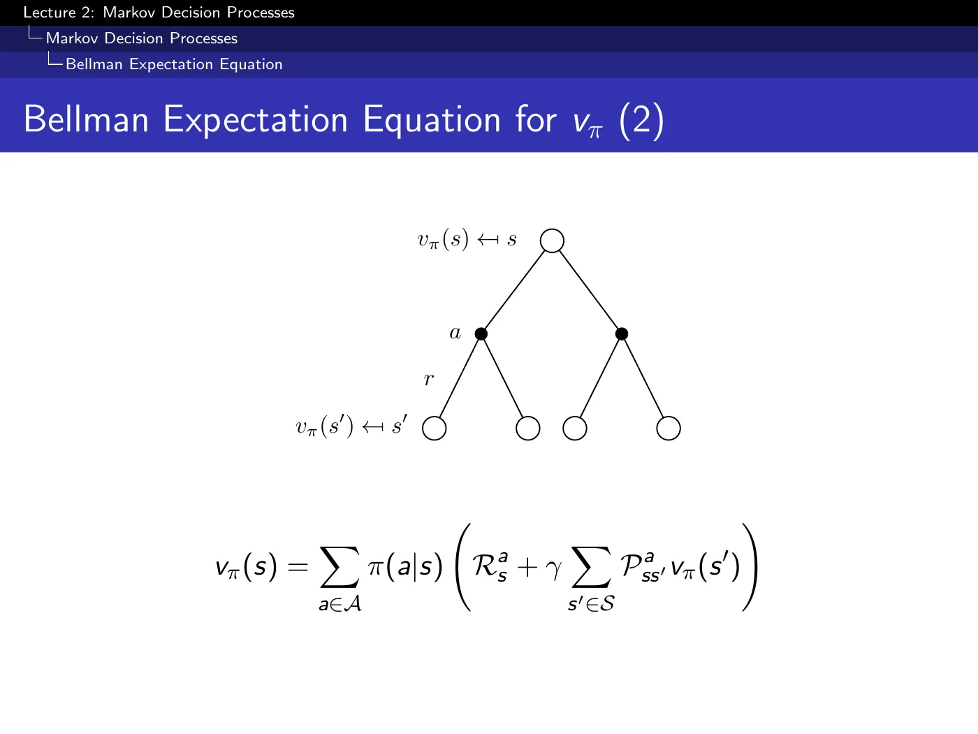
The alternation is the whole structure. Stack the two half-steps and you get the full backup on p.33; stack them the other way and you get p.34. There is no third kind of step in the entire course — later lectures only change how the averages are computed (sampled, approximated) or replace one of them with a max.
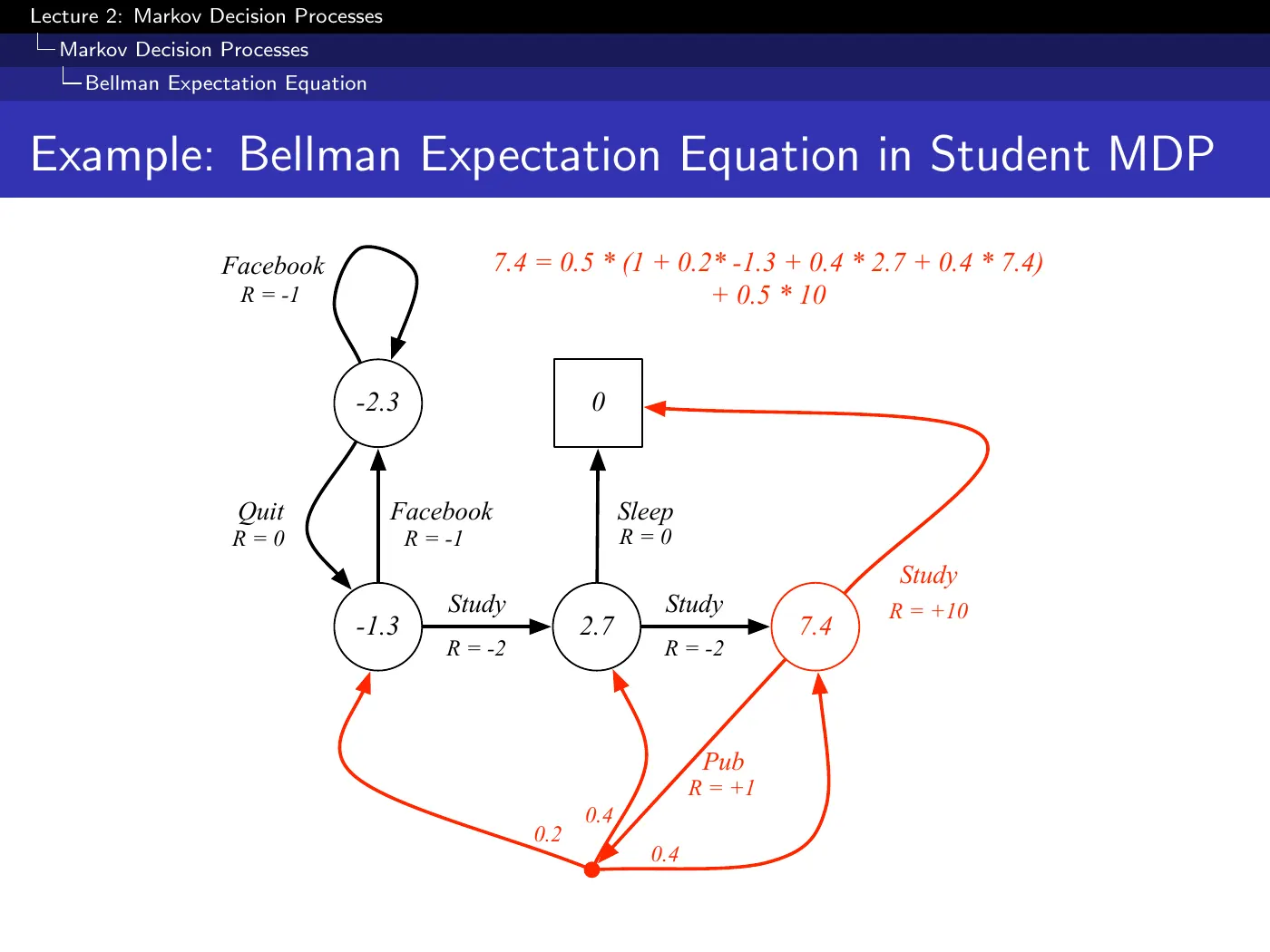
The verification at with uniform:
Note the equation refers to on both sides — the state can reach itself through the pub. Self-consistency, not a computation you could run forward.
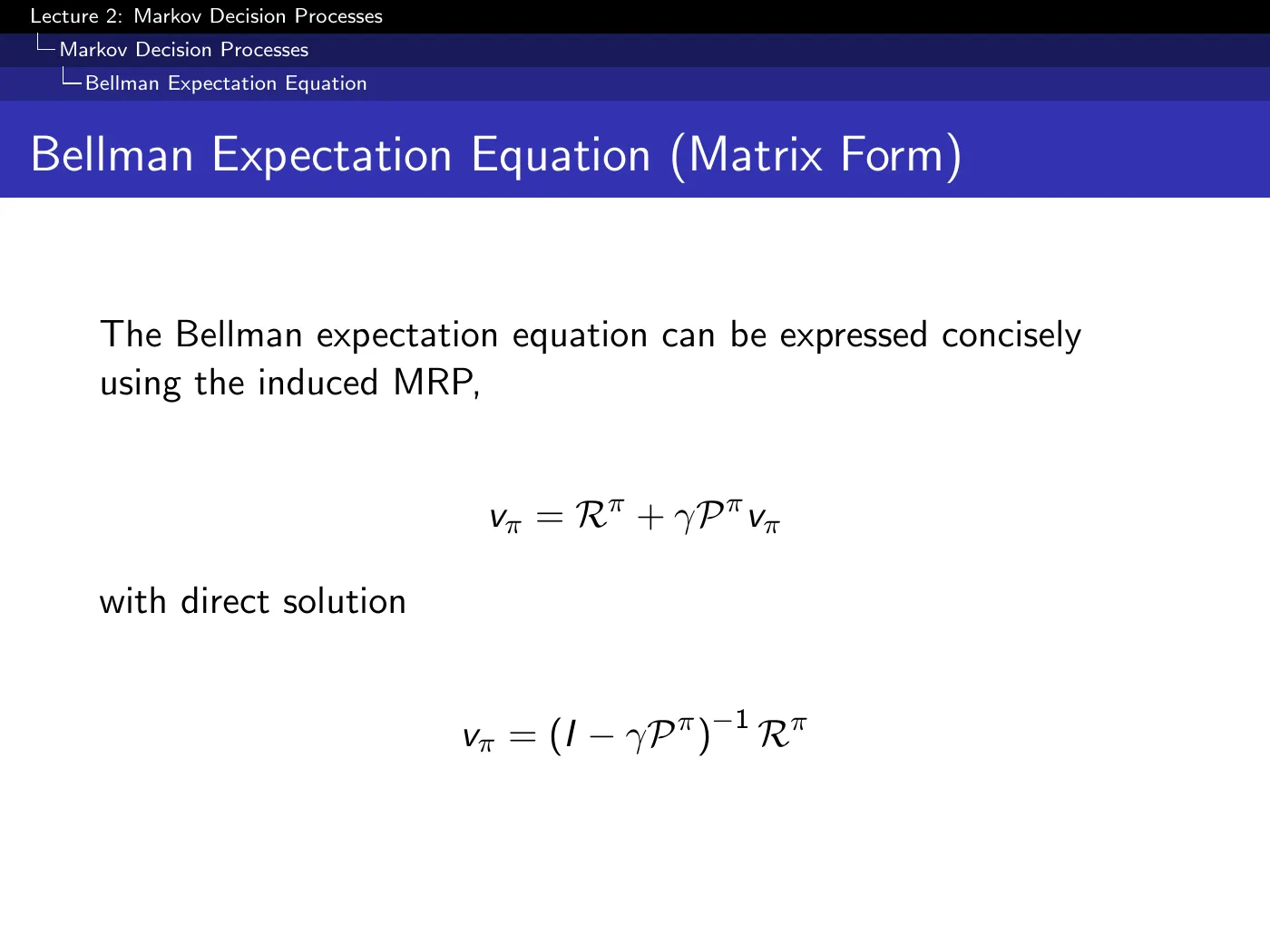
Same linear structure, same closed form, now via the induced MRP: .
6 · Optimality
p.37–39 · Optimal Value Functions ⏱ 1:08:33
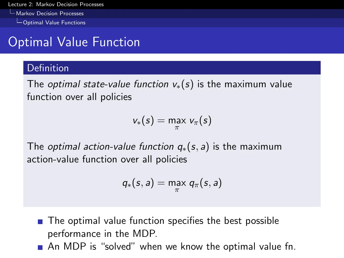
The maximum is over all policies — so tells you the best performance achievable in the MDP, without telling you what achieves it.
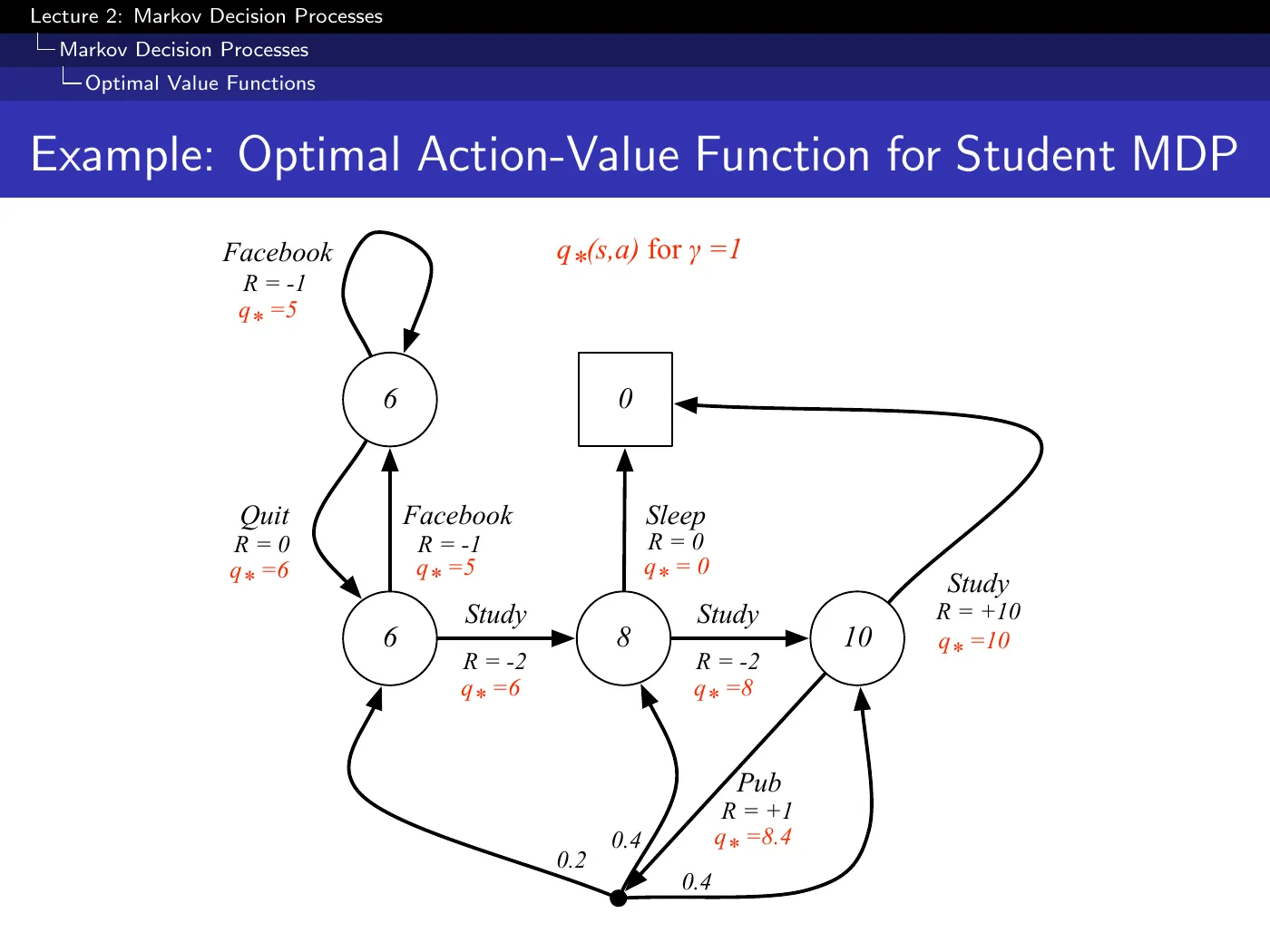
is the transition term alone, without the for going to the pub. The correct value is , and is also what appears in later printings of this deck.
The conclusion is unaffected — studying still wins, — but the margin is much narrower than the slide implies. You caught this yourself by hand-checking → Silver RL Lecture 2 — Question List.
p.40–42 · The Optimal Policy Theorem ⏱ 1:16:07
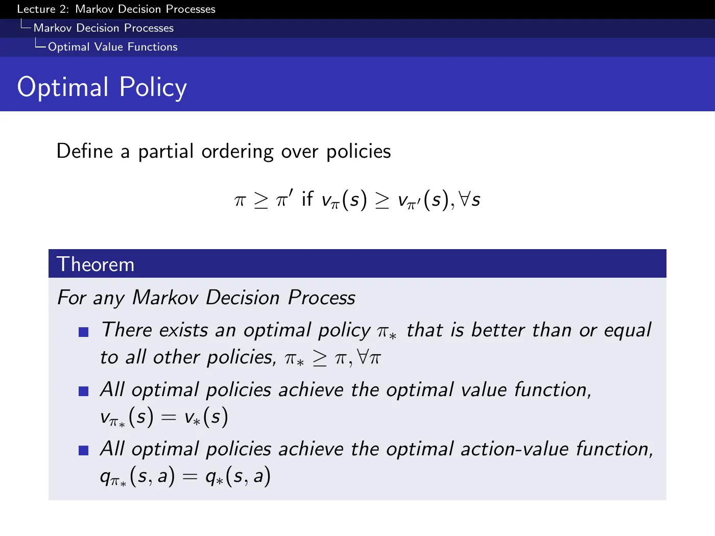
Define iff for all . Note it is a partial order: two policies each better somewhere are simply incomparable.
It rules out the pathology you would otherwise have to worry about: that no single policy dominates, and the best behavior requires switching between policies depending on where you are or how long you have been going.
The theorem says no. There is always at least one that is every other policy simultaneously, in every state. All optimal policies achieve the same and the same — the optimum is unique as a value, even when the policy achieving it is not.
Non-uniqueness is easy: two actions leading to the same state are both optimal. It costs nothing.
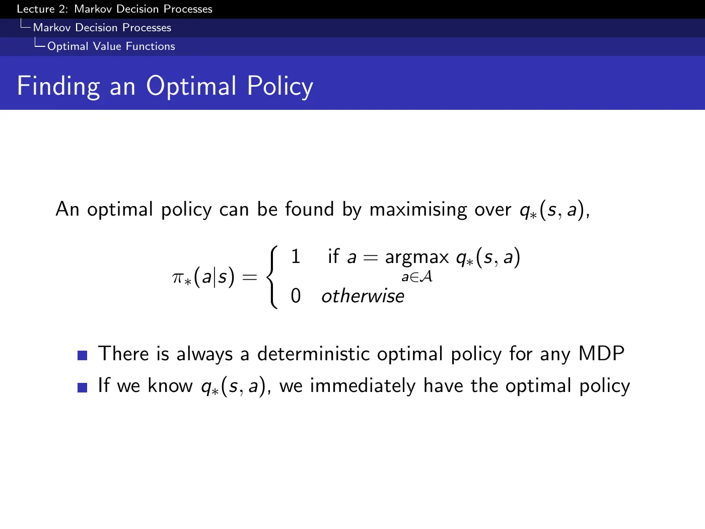
Stochasticity buys you nothing at the optimum: just always take the best action. The search space collapses from all distributions over actions to a finite set of deterministic maps.
Attach the condition, because L7 breaks it. This holds for a Markov, fully observed MDP. Under state aliasing or partial observability the problem is effectively a POMDP, the theorem does not apply, and a stochastic policy can strictly beat every deterministic one → Lecture 7 · Policy Gradient.
And the practical payoff, stated repeatedly: once you have , you are done. Read off the argmax and act. No lookahead, no model, no further computation.
7 · The Bellman optimality equation
p.43–47 · Optimality Backups ⏱ 1:22:57
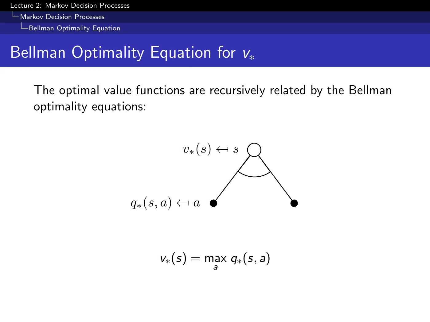
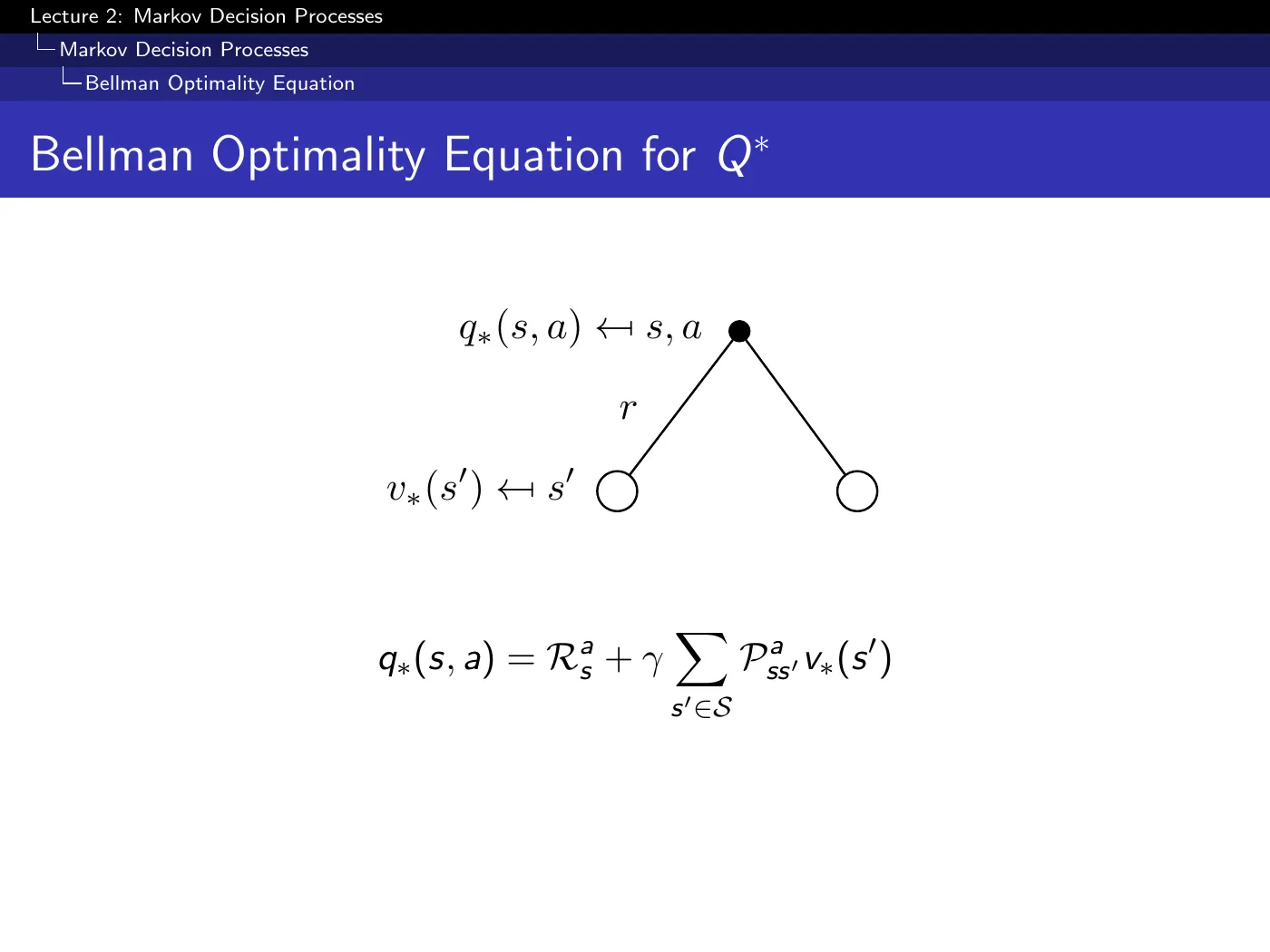
Compare against p.31–32. The step is identical — still an average over , because you never control the environment's dice.
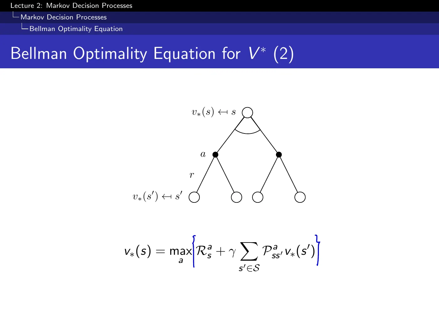
The step changed from to — because now you are choosing, and you choose the best.
Average over what you do not control; maximize over what you do. That sentence is the entire difference between the expectation and optimality equations, and it is why exactly one of the two backup diagrams gained an arc.
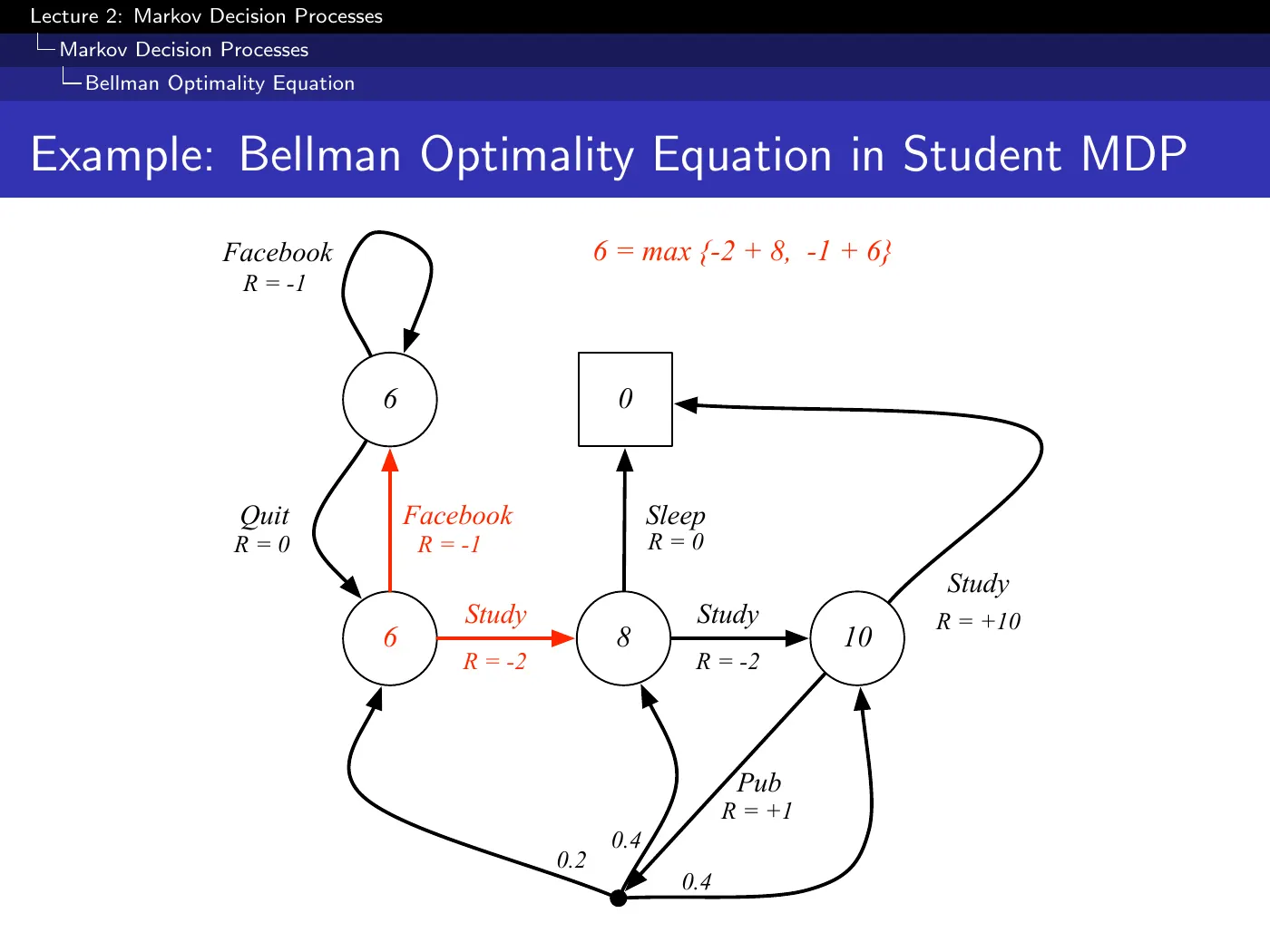
Study gives then a state worth ; Facebook gives then a state worth . The immediate reward is worse and the total is better — a one-line demonstration that greedy on is not myopic, which is the misreading L3 has to correct explicitly.
p.48 · Solving It ⏱ 1:29:52
worked because the expectation equation is linear. The optimality equation has a inside, so it is non-linear, and there is no closed form in general.
The four named replacements are the course: value iteration and policy iteration (L3), Q-learning and Sarsa (L5).
Worth noting what "iterative" means here, since matrix inversion is itself iterative underneath: these methods maintain an estimate of the value function and improve it step by step, rather than performing a fixed numerical routine. That is a different kind of iteration, and it is the one that survives when you no longer know .
Study checklist
Answer these without the notes before moving on to L3. Each item links back to where it is worked out; open the toggle only after you have tried.
1. Give the three layers of the formalism and the question each new ingredient creates.
→ p.24–25 · The MDP ⏱ 43:19
Answer
Markov process — what happens?
Markov reward process — adds reward — how good is it?
Markov decision process — adds actions — what should I do?
Each inherits the layer below, and fixing a policy collapses an MDP back to an MRP, which is why prediction and control separate cleanly.
2. State the Markov property operationally, and say what to do when it fails.
→ p.3–6 · Markov Property and Markov Processes ⏱ 3:05
Answer
— the state is a sufficient statistic of the future, so the history can be discarded.
When it fails, either allow non-stationarity and track the drifting solution, or — better — absorb the missing information into the state. If transition probabilities depend on how long you have been somewhere, that duration is part of the state. "Non-Markov" usually means your state is incomplete.
3. Distinguish from , and give the honest ranking of reasons to discount.
→ p.10–13 · Reward, Return, and Discounting ⏱ 13:04
Answer
is a random variable — one sampled trajectory's discounted reward. is an expectation, a fixed number per state. Averaging sampled estimates — that is Monte-Carlo evaluation, arriving early.
Discounting: (1) mathematically convenient — stated as the real reason; (2) bounds returns in cyclic processes; (3) represents an imperfect model — trusting a ten-year plan means trusting your model that long; (4) interest rates for financial reward; (5) humans and animals genuinely prefer immediate reward. If all sequences terminate, is fine.
4. Derive the Bellman equation for an MRP and say what kind of statement it is.
→ p.19–21 · The Decomposition ⏱ 29:52
Answer
Unroll ; factor out ; recognize the remainder as ; apply the law of iterated expectations to get . Result: .
It is a consistency condition, not a formula. It does not compute ; it characterizes it. Satisfy it everywhere and you have the value function. Every algorithm in L3–L8 forces it to hold.
5. Why can an MRP be solved in closed form, and why does that not settle the subject?
→ p.22–23 · Matrix Form and Direct Solution ⏱ 38:41
Answer
Because the Bellman expectation equation is linear: .
It costs , which is hopeless at scale — and the linearity depended on averaging over a fixed policy. Introduce a and both the linearity and the closed form are gone.
The three named replacements are the rest of the course: dynamic programming, Monte-Carlo, TD learning.
6. What changed between the Student MRP and the Student MDP diagrams?
→ p.24–25 · The MDP ⏱ 43:19
Answer
The state space. Pub was a state; it is now an action. The diagram gained black action-nodes between the white state-nodes, and that is where randomness lives: you choose Pub, then the environment's dice pick , , or .
Every other action has a black dot too, with transition probability 1 — just not drawn. All actions share the same two-stage structure: your choice, then the environment's roll.
7. What are the two half-steps of a backup, and who controls each?
→ p.30–35 · The Backup Diagrams ⏱ 54:51
Answer
(white to black): average over your policy, . You control it.
(black to white): average over the environment, . You do not.
Stack them and you get the full backup. There is no third kind of step in the course — later lectures only change how the averages are computed, or replace one with a max.
8. State the optimal policy theorem and the two conditions worth attaching to it.
→ p.40–42 · The Optimal Policy Theorem ⏱ 1:16:07
Answer
For any MDP there exists for all (with meaning in every state), all optimal policies achieve and , and there is always a deterministic optimal policy.
It rules out needing to switch policies depending on where you are — a single policy dominates everywhere at once.
Conditions: the order is partial, so incomparable policies exist; and determinism holds for a Markov, fully observed MDP. Under aliasing or partial observability the theorem does not apply and a stochastic policy can strictly win (L7).
9. Write both Bellman equations for and say precisely what differs.
→ p.43–47 · Optimality Backups ⏱ 1:22:57
Answer
Expectation: .
Optimality: .
Exactly one half-step changed. The step is identical — still an average over , because you never control the dice. The step went from to , because now you are choosing.
Average over what you do not control; maximize over what you do.
10. Why is solving an MDP defined as finding rather than ?
→ p.37–39 · Optimal Value Functions ⏱ 1:08:33
Answer
tells you how much reward is available but not how to get it — choosing would still need a one-step lookahead through and , i.e. a model.
finishes the job: , no model needed. Once you have , read off the argmax and act.
This is exactly the argument L5 reconstructs as its first substitution () when it removes the model.
11. Why is there no closed-form solution to the Bellman optimality equation?
→ p.48 · Solving It ⏱ 1:29:52
Answer
The makes it non-linear. worked only because the expectation equation was linear in .
The replacements named on the slide are the course: value iteration and policy iteration (L3), Q-learning and Sarsa (L5).
"Iterative" here means maintaining an estimate of the value function and improving it step by step — not a numerical routine for a fixed computation. That is the kind of iteration that survives losing .
12. The slide says . Check it.
→ p.37–39 · Optimal Value Functions ⏱ 1:08:33
Answer
.
is the transition term with the immediate reward dropped. The decision is unchanged — studying gives — but the margin is far narrower than the slide suggests, and appears in later printings.
Gaps to close on your own
The lecture runs out of time and takes questions instead. The slides are marked (no exam), but two of the three blocks matter a great deal for where you are going.
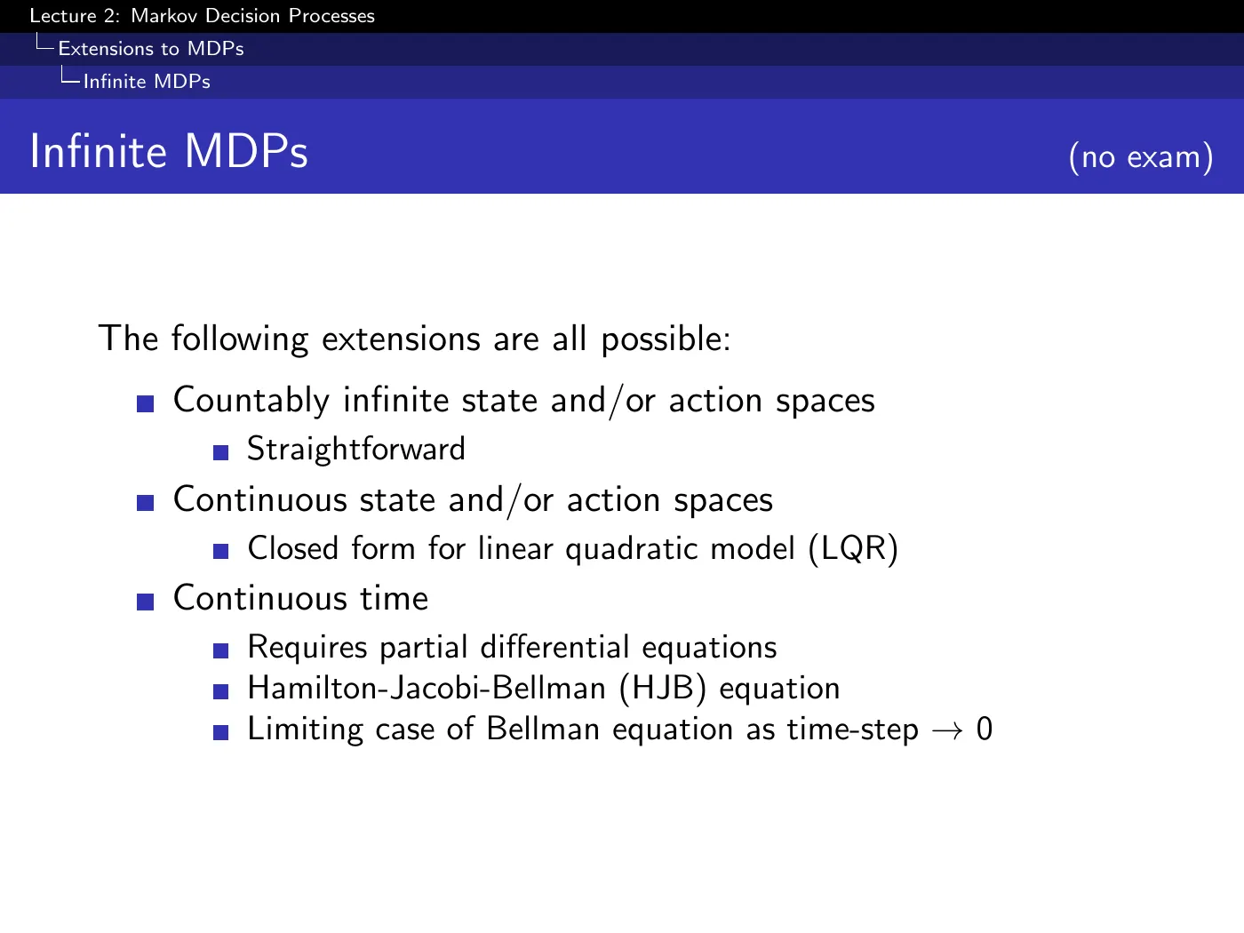
Infinite MDPs. Countably infinite spaces are straightforward; continuous state and action spaces have a closed form in the linear-quadratic case (LQR); and continuous time requires PDEs, giving the Hamilton-Jacobi-Bellman equation — the limiting case of the Bellman equation as the time-step goes to zero.
This is the bridge between this course and classical optimal control, and the reason "RL and control are the same subject in different notation" is more than a slogan → LQR and the Riccati Equation · Hamilton-Jacobi-Bellman (HJB) · your own Silver RL Lecture 2 — Question List Q5.
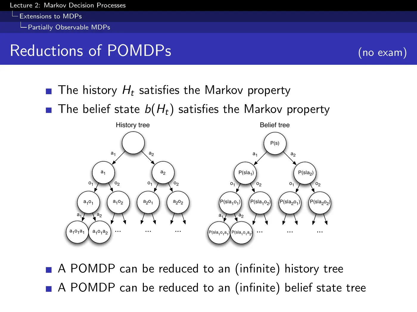
POMDPs. A POMDP adds observations and an observation function . The key result is on this slide: both the history and the belief state satisfy the Markov property, so a POMDP reduces to an (infinite) MDP over either. That is the precise sense in which "partially observable problems can be converted into MDPs" from p.3 — and the belief-state tree is the direct ancestor of L9's information-state search.
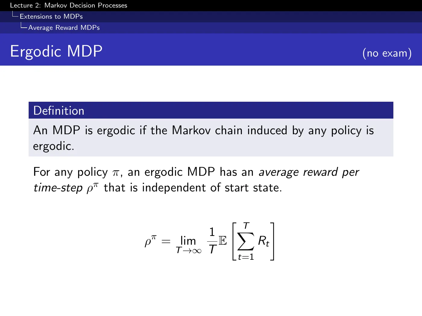
Average-reward MDPs. For an ergodic MDP (recurrent + aperiodic), there is a stationary distribution and an average reward per step independent of the start state, with its own Bellman equation in terms of . This is the principled alternative to discounting for continuing problems, and reappears as the state distribution in L7's policy objectives.
- Technical conditions for undiscounted MDPs. The lecture defers to Bertsekas (Dynamic Programming and Optimal Control, vol. 2) for when undiscounted MDPs are well defined. If you ever want without guaranteed termination, this is the gap.
- The optimal policy theorem is stated, not proved. Your own Silver RL Lecture 2 — Question List Q3 already asked whether the proof is worth knowing; the proof itself is in Puterman or Sutton & Barto.
- Why the Bellman equation has a unique solution is assumed throughout and answered in L3 by the contraction mapping theorem → Contraction Mapping & Bellman Convergence.
- Sherman-Morrison for incremental matrix inversion is mentioned as reducing to in special cases. It returns in L6 for LSTD.
Language notes
Phrasings worth stealing for your own technical writing and talks:
| Expression | Use |
|---|---|
| the future is independent of the past given the present | the Markov property in one sentence |
| a sufficient statistic of the future | a compression that loses nothing predictive |
| how much juice you can extract | informal gloss on optimal value |
| value judgments | rewards, framed as the modeller's choice rather than a fact |
| maximally shortsighted / maximally farsighted | the two ends of a discount factor |
| you have to really trust your model | why long-horizon plans get discounted |
| the environment rolls the dice | the stochastic half of a transition |
| this is a sanity theorem | a result confirming everything you hoped was true |
| once we have we're done, the game is solved | naming the terminal goal of a formalism |
| don't confuse yourselves, it's just a convention | flagging notation as arbitrary before it derails someone |