Lecture 6 · Value Function Approximation

Slides: David Silver - RL Course (UCL 2015) · Previous: Lecture 5 · Model-Free Control · Next: Lecture 7 · Policy Gradient

First pass: read The one idea and the slide-group headings. Use the prose when an equation, condition, or figure needs explanation; leave Gaps to close for review.

The one idea

L1–L5 all assumed one thing without ever stating it: a lookup table. One cell per state, or per state-action pair. L6 removes that assumption and replaces the table with a parameterized function, then asks the only question that matters — does everything still work?

The answer splits cleanly, and the split organizes the whole lecture:

	Table lookup (L1–L5)	Function approximation (L6)
Representation	$V(s)$ , $Q(s,a)$ — one cell each	$\hat v(s,\mathbf{w})$ , $\hat q(s,a,\mathbf{w})$ — one shared $\mathbf{w}$
Update	overwrite a cell	move $\mathbf{w}$ along a gradient
Side effect on other states	none	generalization — the whole point
MC prediction	tabular estimate	SGD on a fixed regression target; linear is the cleanly guaranteed case
TD prediction	converges under the usual tabular assumptions	on-policy linear TD converges; ordinary TD can diverge off-policy or with non-linearity
Control	converges under the usual exploration and step-size assumptions	approximate improvement may chatter; some combinations can diverge

The method of the whole lecture — pretend, then substitute

Every derivation here runs in two stages. Stage 1: assume an oracle hands you the true $v_\pi(S)$ , and derive the supervised-learning update. Stage 2: paste an RL target where the oracle was — the return $G_t$ , the TD target $R+\gamma\hat v(S',\mathbf{w})$ , or the $\lambda$ -return $G_t^\lambda$ .
The lecture runs this exact loop three times: for prediction (p.12→16), for control (p.22→24), and for least squares (p.42→45). Once you see the pattern, two-thirds of the slides are the same slide.

One-hot features $x_\text{table}(S)=\big(\mathbf{1}(S=s_1),\dots,\mathbf{1}(S=s_n)\big)^\top$ turn linear function approximation into a lookup table (p.15). Nothing from L1–L5 is discarded. A table is simply the corner case in which different states share no active features, so an update at one state cannot generalize to another.

Core map — what must survive L6

Why approximation: a table is impossible in huge or continuous state spaces, but the deeper benefit is generalization and data efficiency.
Linear means linear in the parameters: $\hat v(s,\mathbf w)=x(s)^\top\mathbf w$ may use highly non-linear features $x(s)$ . One-hot $x(s)$ recovers table lookup.
One update pattern: $\Delta\mathbf w=\alpha\big(\text{target}-\hat v\big)\nabla_\mathbf w\hat v.$ Start with the unavailable target $v_\pi$ , then substitute $G_t$ , $R_{t+1}+\gamma\hat v(S_{t+1},\mathbf w)$ , or $G_t^\lambda$ .
MC versus TD: the MC target is independent of the current parameters, so the update is genuine SGD on a fixed prediction objective. A bootstrapped TD target also contains $\mathbf w$ ; ordinary TD ignores that target derivative and is therefore a semi-gradient method.
Control uses $\hat q(s,a,\mathbf w)$ : Sarsa bootstraps from the next action sampled under the current policy; Q-learning bootstraps from $\max_{a'}\hat q(S',a',\mathbf w)$ . Approximation error can make a nominal policy-improvement step fail to improve.
Bootstrapping is useful but creates feedback: intermediate $\lambda$ often beats pure MC because it lowers variance. Instability becomes especially dangerous when bootstrapping, shared function approximation, and off-policy data interact — the deadly triad. This is a risk pattern, not an if-and-only-if theorem.
DQN is approximate Q-learning with a neural-network $Q$ : the network learns both representation and values. Experience replay reduces temporal correlation and reuses data; a target network slows target drift. Neither device removes the deadly triad or proves convergence.
Batch alternatives reuse a fixed dataset: LSMC uses MC targets, LSTD uses TD fixed-point equations, and LSPI alternates LSTDQ evaluation with greedy improvement on the same batch.

1 · Why approximate at all
2 · The oracle assumption
3 · Removing the oracle — prediction
4 · Control
5 · When it breaks
6 · Batch methods
7 · DQN
8 · Closed-form least squares
Study checklist
Gaps to close on your own
Language notes

1 · Why approximate at all

p.4–5 · Large-Scale Reinforcement Learning ⏱ 1:36

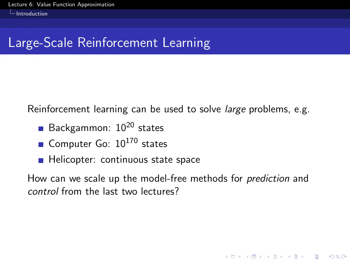
Lecture 6 Value Function Approximation, slide 5

Backgammon $10^{20}$ , Go $10^{170}$ , helicopter uncountably infinite. The numbers are there to rule out the table, but the argument they make is the weaker of the two reasons to approximate.

The stronger reason is on the next slide and is easy to read past: even with infinite memory, learning a separate value for the state you are in and the state one millimeter to the right is hopeless — you would need a separate trajectory through each. Approximation is a statement about data efficiency before it is a statement about memory.

p.6 · Value Function Approximation ⏱ 3:58

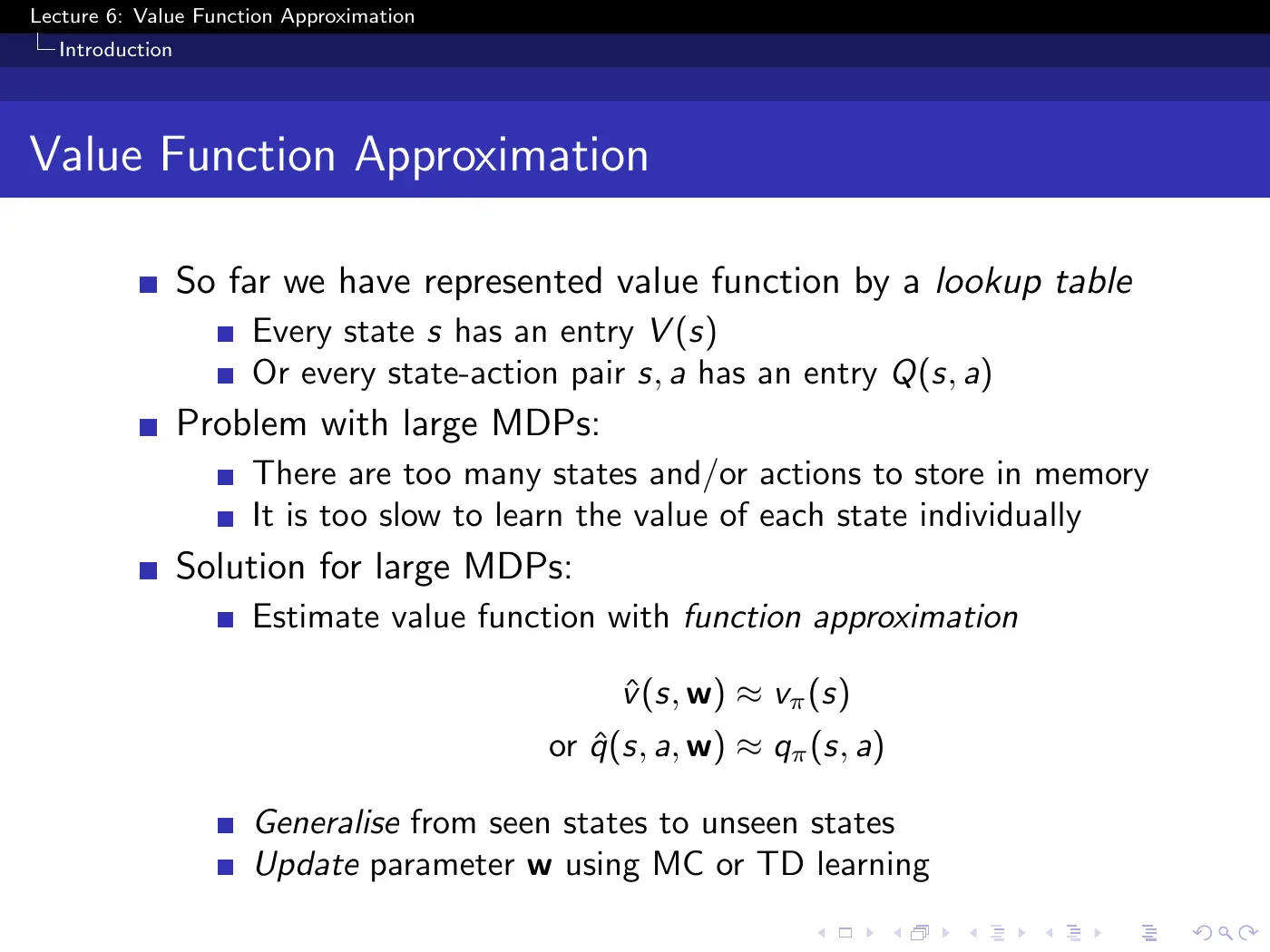
Lecture 6 Value Function Approximation, slide 6

\hat v(s,\mathbf{w})\approx v_\pi(s)\qquad\text{or}\qquad \hat q(s,a,\mathbf{w})\approx q_\pi(s,a)

Two distinct wins, and the slide lists them as one bullet each without ranking them:

Memory — $\dim(\mathbf{w}) \ll |\mathcal{S}|$ .
Generalization — you can query the approximator at states you have never visited.

Win 2 is the one that makes RL possible at scale. Win 1 alone would be worthless: a compressed table you can only read at visited entries is still a table.

The last bullet is the entire second half of the lecture in six words — update $\mathbf{w}$ using MC or TD. No new learning principle is introduced today. Only a new representation.

p.7 · Types of Value Function Approximation ⏱ 8:30

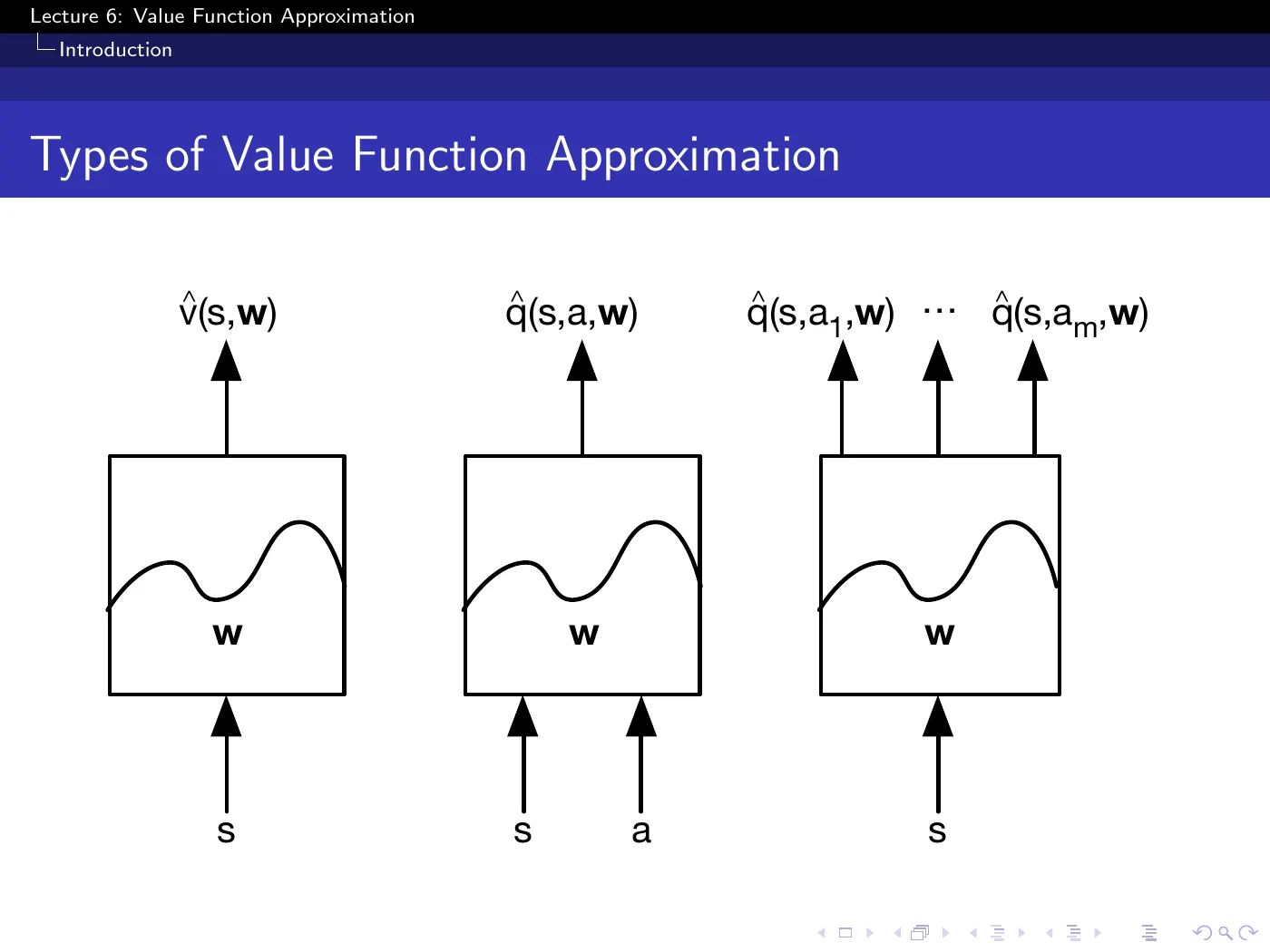
Lecture 6 Value Function Approximation, slide 7

Three architectures. The two on the right are action-in and action-out, and the choice is not cosmetic:

	Input	Output	Cost of $\arg\max_a$
Action-in	$(s,a)$	one scalar $\hat q(s,a,\mathbf{w})$	one forward pass per action
Action-out	$s$	a vector $\hat q(s,a_1,\mathbf{w}),\dots,\hat q(s,a_m,\mathbf{w})$	one forward pass total

They represent the same information but train differently and cost differently. Since control needs $\arg\max_a \hat q$ at every single step, action-out is what makes greedy action selection cheap — and it is exactly what DQN uses on p.39, emitting all 18 joystick values in one pass.

Action-out has a hidden precondition

It requires a finite, fixed, discrete action set, since the output layer has one unit per action. Action-in has no such constraint and scales to large or continuous action spaces — but then $\max_a$ stops being a lookup and becomes an optimization problem in its own right. This limitation resurfaces at Mountain Car (p.25) and is one of the reasons L7 turns to policy-based methods.

p.8–9 · Which Function Approximator ⏱ 11:57

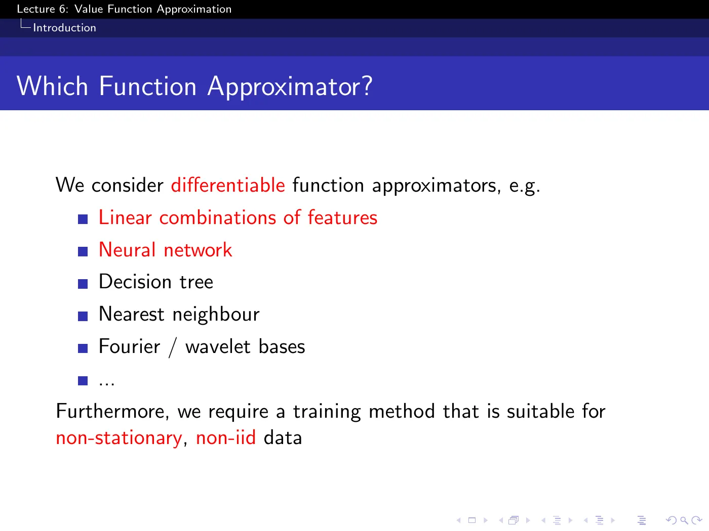
Lecture 6 Value Function Approximation, slide 9

Two requirements are being imposed here, and they are different in kind.

Differentiability is a convenience — it buys the gradient toolkit and hence cheap incremental updates.

Suitability for non-stationary, non-i.i.d. data is the RL-specific constraint, and it is the thesis statement for everything after p.33:

Non-stationary — the target moves. In control $\pi$ improves, so $v_\pi$ itself changes shape. Even in pure prediction the TD target moves, because it is computed from the same $\mathbf{w}$ you are updating.
Non-i.i.d. — data arrives as trajectories, and where you are now is heavily correlated with where you will be next.

Hold onto both words. DQN's two tricks (p.38) map onto them one-for-one: experience replay attacks non-i.i.d., fixed Q-targets attack non-stationarity.

The bullet list on p.9 is stale

It is the p.8 list copy-pasted under a new heading. Decision trees and nearest neighbor are not differentiable, so they do not belong under "we consider differentiable function approximators." The lecture treats linear combinations of features as the canonical case and neural networks as the non-linear case, and nothing else appears again.

2 · The oracle assumption

p.11–12 · Value Function Approximation by SGD ⏱ 15:30

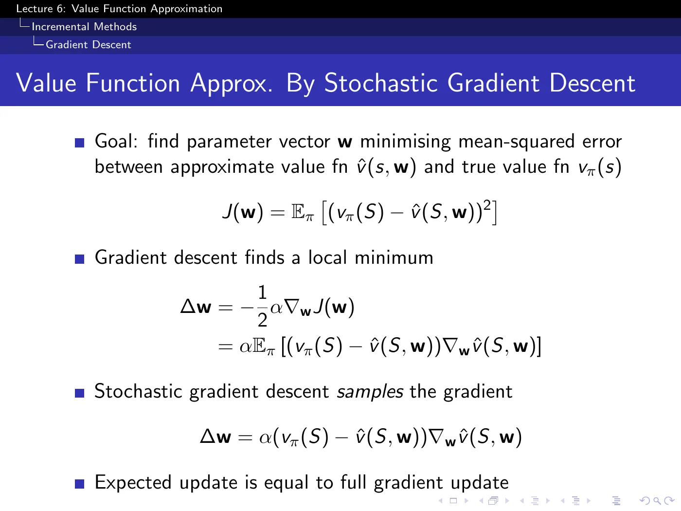
Lecture 6 Value Function Approximation, slide 12

J(\mathbf{w})=\mathbb{E}_\pi\big[(v_\pi(S)-\hat v(S,\mathbf{w}))^2\big] \qquad\Longrightarrow\qquad \Delta\mathbf{w}=\alpha\big(v_\pi(S)-\hat v(S,\mathbf{w})\big)\nabla_\mathbf{w}\hat v(S,\mathbf{w})

The $\tfrac{1}{2}$ in $-\tfrac{1}{2}\alpha\nabla_\mathbf{w}J(\mathbf{w})$ is bookkeeping — it cancels the $2$ from differentiating the square. Read no meaning into it.

This slide rests on an assumption RL cannot make, and says so only in the first bullet. $v_\pi(S)$ is assumed given by an oracle, which is precisely what RL does not have. Everything derived here is therefore provisional until p.16 replaces the oracle.

Note where the gradient lands: the oracle term is a constant with respect to $\mathbf{w}$ , so differentiating the squared error leaves $\nabla_\mathbf{w}\hat v$ alone. That is trivially true here. It stops being trivially true the moment the oracle is replaced by a bootstrap target — see p.18.

The last line, "expected update is equal to full gradient update", is what licenses the online algorithm. You never compute the expectation over the state distribution; you visit states according to $\pi$ and let the visitation itself perform the averaging.

p.13–14 · Feature Vectors and Linear Value Function Approximation ⏱ 22:06

Lecture 6 Value Function Approximation, slide 14

\hat v(S,\mathbf{w})=x(S)^\top\mathbf{w},\qquad \nabla_\mathbf{w}\hat v(S,\mathbf{w})=x(S),\qquad \Delta\mathbf{w}=\alpha\big(v_\pi(S)-\hat v(S,\mathbf{w})\big)\,x(S)

\text{Update}=\underbrace{\alpha}_{\text{step size}}\times\underbrace{\big(v_\pi(S)-\hat v(S,\mathbf{w})\big)}_{\text{prediction error}}\times\underbrace{x(S)}_{\text{credit assignment}}

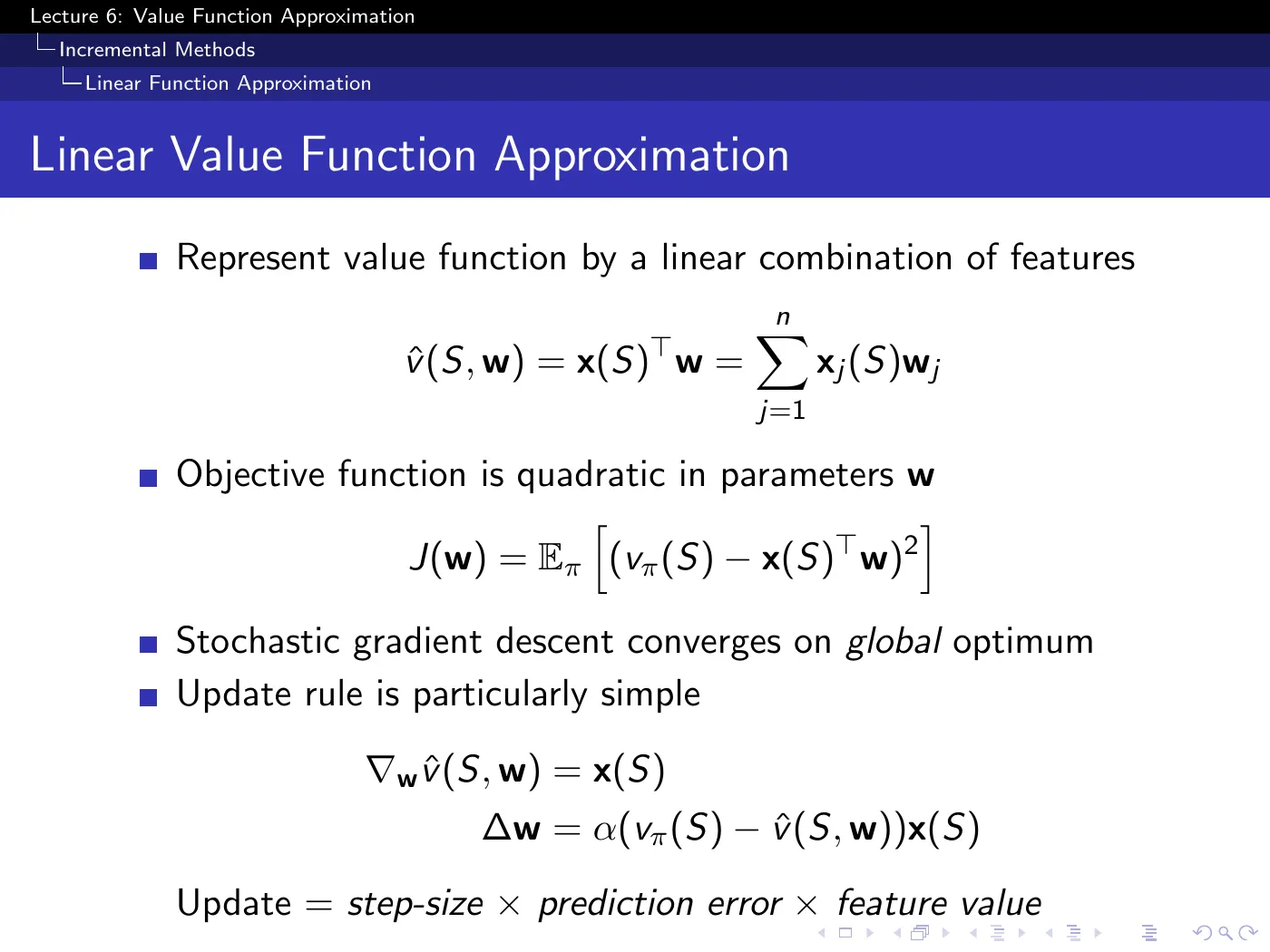
The third factor is the interesting one, and the slide reduces it to the flat phrase "feature value." What it actually does is assign credit: a feature that is off contributes nothing to the update of its weight. If you are holding a position with no queen and your evaluation turns out to be wrong, you do not adjust the queen weight — that feature had nothing to do with the error.

"Linear" means linear in

\mathbf{w}

, not linear in the state

$J(\mathbf{w})$ is quadratic and convex in the parameters, so it has no suboptimal local minima. The minimizing parameter vector is unique only when the feature covariance has full rank; otherwise several vectors can represent the same best prediction. The features $x(S)$ themselves may be arbitrarily non-linear functions of the state — Gaussians, tile codings, wavelets, polynomial terms.
This is not a technicality. Mountain Car (p.25–26) uses coarse coding and radial basis functions and is still, in this lecture's sense, linear function approximation, so the relevant linear-theory results can apply when their other assumptions hold.

Features are lossy by design. You are choosing to throw away everything that distinguishes two states with identical feature vectors — and if the features are good, that discarded information was not needed. The lecture does not address where good features come from; that is the representation-learning problem, and the answer it points to is use a neural network and stop hand-designing them.

p.15 · Table Lookup Features ⏱ 28:57

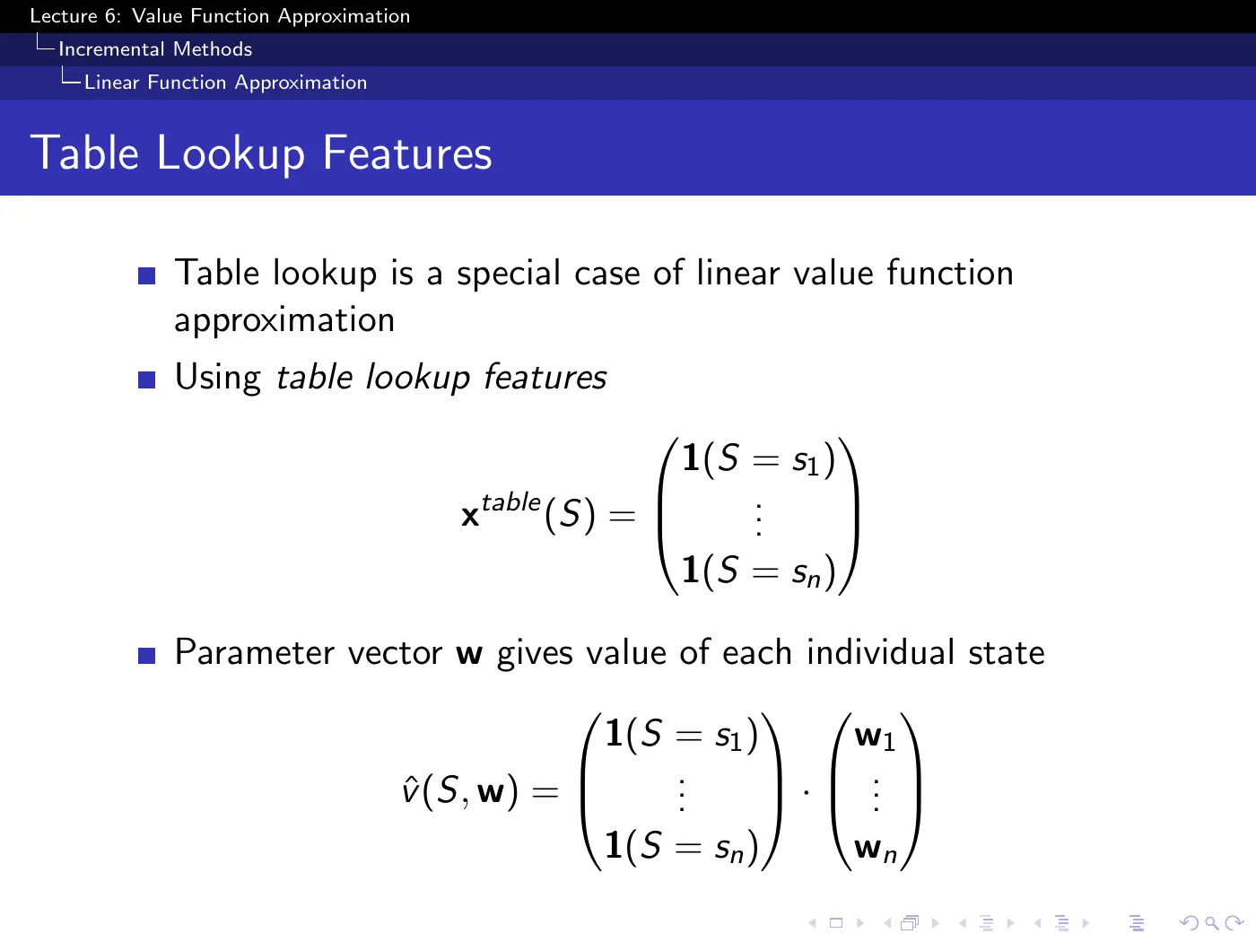
Lecture 6 Value Function Approximation, slide 15

With one-hot features the dot product selects a single weight, so $\mathbf{w}$ is the table. Everything from the last five lectures is a special case of today.

The more useful reading is the contrapositive. In this encoding no two states share any active feature, so an update to one state's weight moves no other state's value by exactly zero. That is the precise sense in which a table cannot generalize, and it identifies what generalization actually is: overlap between the feature vectors of different states. Coarse coding works because nearby states light up shared tiles.

3 · Removing the oracle — prediction

p.16 · Incremental Prediction Algorithms ⏱ 31:16

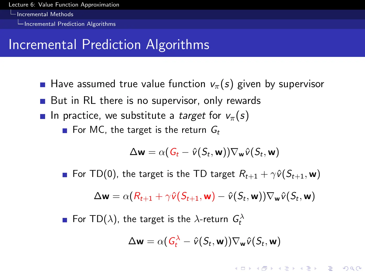
Lecture 6 Value Function Approximation, slide 16

The oracle assumed on p.12 is replaced by substitution — three targets, one update rule:

\text{MC:}\ \ \Delta\mathbf{w}=\alpha\big(G_t-\hat v(S_t,\mathbf{w})\big)\nabla_\mathbf{w}\hat v(S_t,\mathbf{w})

\text{TD(0):}\ \ \Delta\mathbf{w}=\alpha\big(R_{t+1}+\gamma\hat v(S_{t+1},\mathbf{w})-\hat v(S_t,\mathbf{w})\big)\nabla_\mathbf{w}\hat v(S_t,\mathbf{w})

\text{TD}(\lambda)\text{:}\ \ \Delta\mathbf{w}=\alpha\big(G_t^{\lambda}-\hat v(S_t,\mathbf{w})\big)\nabla_\mathbf{w}\hat v(S_t,\mathbf{w})

The slide presents these as three equally-good options. They are not, and the difference is the root of the entire convergence section:

Target	Biased?	Depends on $\mathbf{w}$ ?	Consequence
$G_t$	no — unbiased	no	genuinely SGD on a fixed objective
$R_{t+1}+\gamma\hat v(S_{t+1},\mathbf{w})$	yes	yes	not generally gradient descent on a fixed prediction loss
$G_t^\lambda$	generally yes for $\lambda<1$	yes for $\lambda<1$	semi-gradient; at $\lambda=1$ it reduces to MC

The second column is the familiar bias-variance story. The third column reveals the new stability issue: parameter-dependent bootstrap targets create feedback, and the semi-gradient update does not inherit ordinary SGD's objective-descent guarantee. That is what makes divergence possible, as p.31 states explicitly.

p.17 · Monte-Carlo with Value Function Approximation ⏱ 35:05

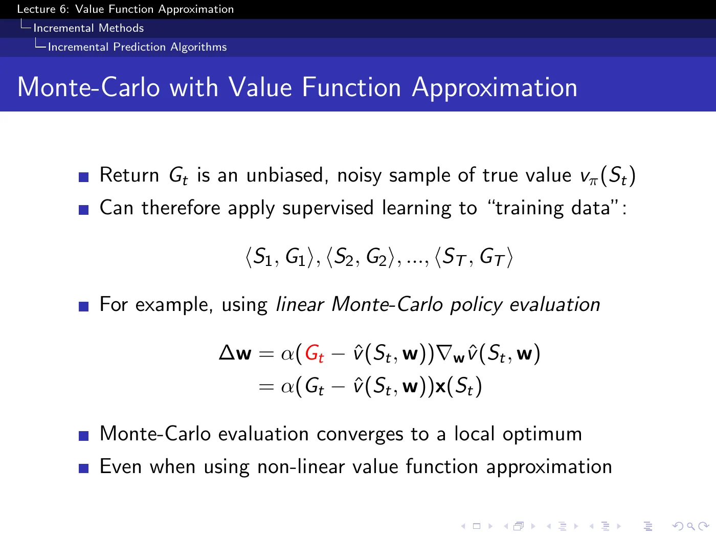
Lecture 6 Value Function Approximation, slide 17

$G_t$ is an unbiased sample of $v_\pi(S_t)$ , so MC is supervised learning with a noisy oracle. This explains the ✓ marks in the MC row of the lecture's convergence tables. The target does not depend on $\mathbf{w}$ , so the update is stochastic gradient descent on a fixed prediction objective; convergence still requires the usual sampling, step-size, and smoothness assumptions. In the linear case the objective is convex; in the non-linear case even a stationary point need not be globally optimal.

The price is variance, and it is severe enough that p.27 shows MC losing to bootstrapping on every benchmark.

p.18 · TD Learning with Value Function Approximation ⏱ 37:24

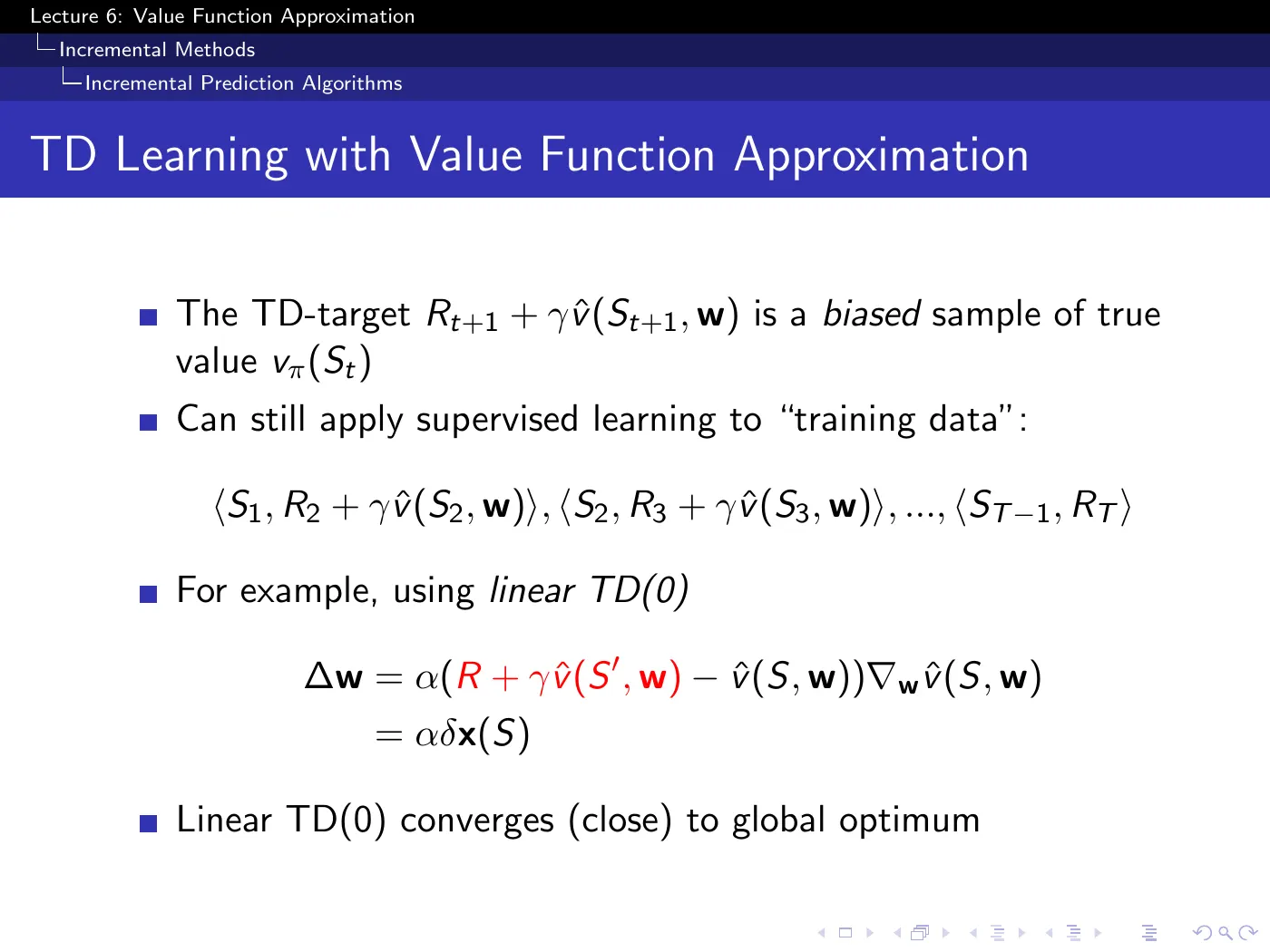
Lecture 6 Value Function Approximation, slide 18

\Delta\mathbf{w}=\alpha\,\delta\,x(S),\qquad \delta=R+\gamma\hat v(S',\mathbf{w})-\hat v(S,\mathbf{w})

The slide's last line — "Linear TD(0) converges (close) to global optimum" — hides its most important word in parentheses. TD(0) converges to the TD fixed point $\mathbf{w}_{TD}=A^{-1}b$ , which is not the least-squares optimum. The gap is bounded (Tsitsiklis & Van Roy, 1997; Sutton & Barto 2e eq. 9.14, proved for the continuing case):

\overline{VE}(\mathbf{w}_{TD})\;\le\;\frac{1}{1-\gamma}\min_{\mathbf{w}}\overline{VE}(\mathbf{w})

Read the size of that constant before trusting the tick mark

$\frac{1}{1-\gamma}$ is not a small correction. At $\gamma=0.99$ it is 100 — the TD solution is guaranteed only to be within two orders of magnitude of the best representable one, and $\gamma$ near 1 is the normal case.
The bound is worst-case and TD usually does far better in practice, but "converges close to the global optimum" is doing much more work than the phrase suggests. What you get in return is variance: TD is typically far faster than MC, which attains the $\min$ but slowly.

The "training data" framing is conceptual, not literal

Both p.17 and p.18 display a dataset $\langle S_1, G_1\rangle,\dots$ as though you collect it and then run supervised learning. You do not — not in this half of the lecture. Every update is applied online, one step at a time, and the experience is discarded immediately afterwards. The dataset only becomes a real stored object at p.36, which is exactly what makes batch methods a different thing.

The TD target also contains

\mathbf{w}

. Why does the gradient apply only to

\hat v(S,\mathbf{w})

and not to both terms?

Because TD is designed as a stochastic approximation to a Bellman fixed point, not as ordinary regression on a fixed label. It freezes the bootstrap target for that update and changes only the current-state prediction. That deliberate omission makes it a semi-gradient method.

Differentiating the squared TD error through both predictions gives a different family, usually called residual-gradient methods. In stochastic environments, an unbiased sample of that full gradient generally requires two independent next-state samples from the same $(s,a)$ — the double-sampling problem. Ordinary TD avoids that requirement, but gives up the safety of following the gradient of a fixed scalar objective.

p.19–20 · TD(λ) with Value Function Approximation ⏱ 41:59

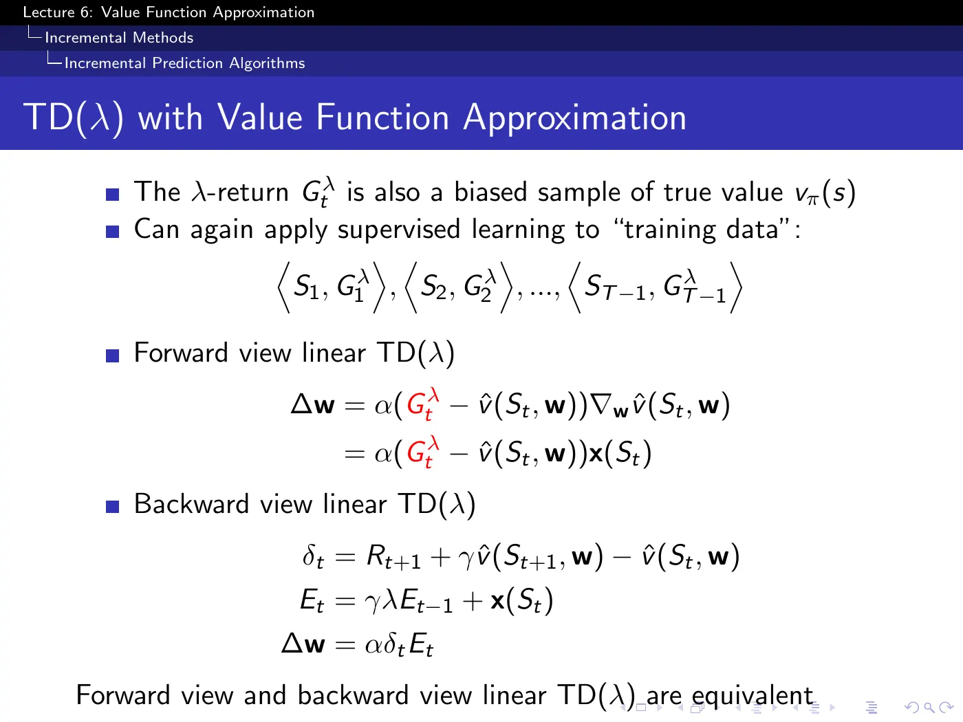
Lecture 6 Value Function Approximation, slide 20

\delta_t=R_{t+1}+\gamma\hat v(S_{t+1},\mathbf{w})-\hat v(S_t,\mathbf{w}),\qquad E_t=\gamma\lambda E_{t-1}+x(S_t),\qquad \Delta\mathbf{w}=\alpha\,\delta_t E_t

The forward and backward views have the same episodic/offline equivalence developed in L4 → Forward and Backward Views of TD Lambda. With weights changing online, exact step-by-step equivalence requires the true-online correction; the conventional trace is an online approximation to the interim forward view.

The eligibility trace now lives on the parameters, not on the states

$E_t$ has the dimension of $\mathbf{w}$ — one entry per feature, not one per state-action pair. In L5 the trace was an $|\mathcal{S}|\times|\mathcal{A}|$ table the same size as $Q$ , which would have been just as unusable at scale as $Q$ itself.
This is the small change that makes traces survive the transition to function approximation, and it is easy to miss because the update equation looks unchanged. The trace accumulates feature vectors, so credit is assigned to whichever features were active and in proportion to how strongly — the same recency-and-frequency heuristic as L5, re-expressed per feature.

4 · Control

p.21 · Control with Value Function Approximation ⏱ 49:04

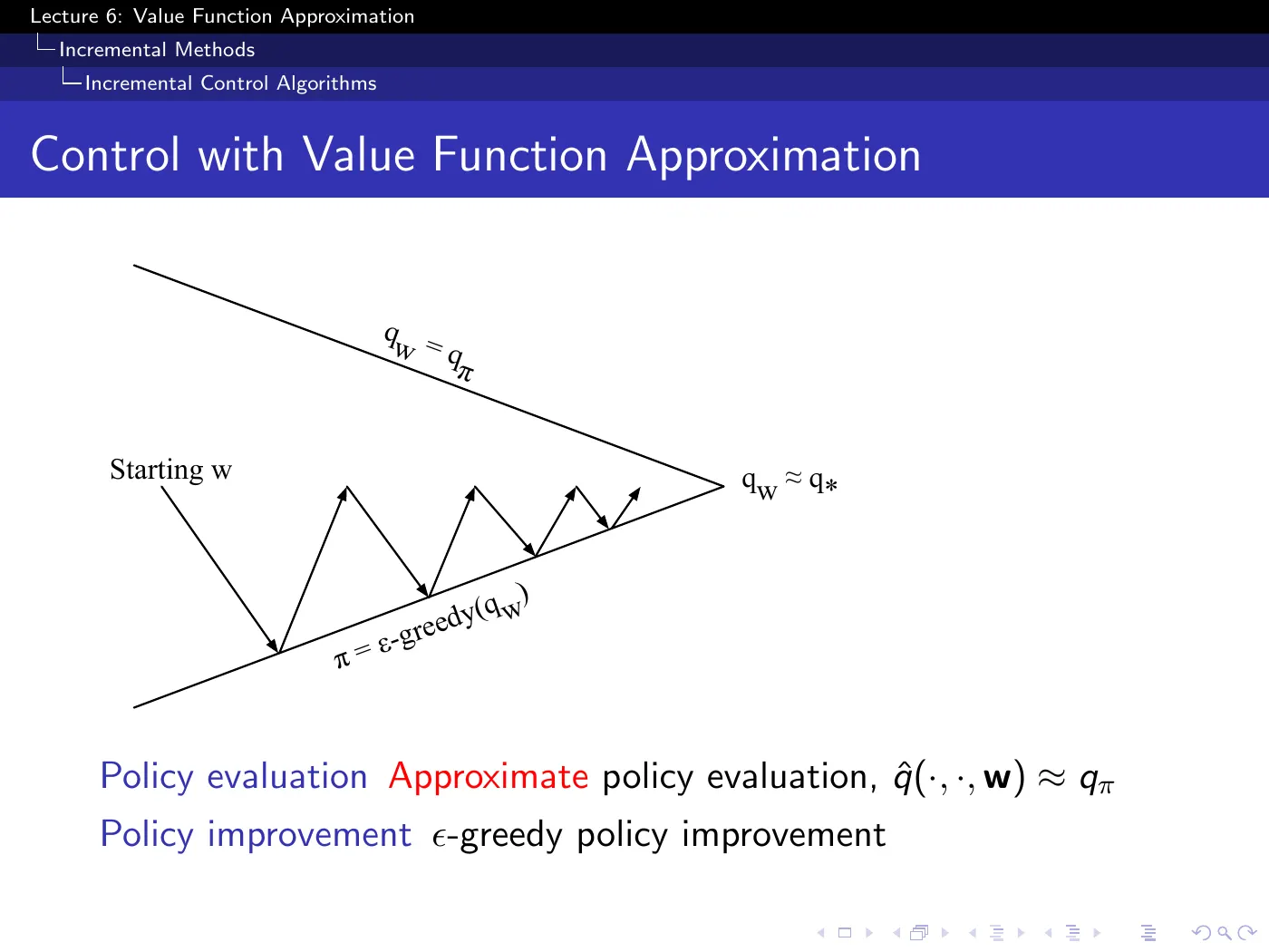
Lecture 6 Value Function Approximation, slide 21

The same GPI loop as L5, with approximate evaluation in the up-arrow and $\epsilon$ -greedy improvement in the down-arrow. As in L5, do not run evaluation to convergence before improving — act on the freshest estimate, which in the fully incremental case means updating and re-acting every single step.

Read the diagram's two labels differently

The top label $\hat q_\mathbf{w}=q_\pi$ should be read as the evaluation goal, not a promise. Equality is possible only when the chosen function class can represent $q_\pi$ and the learning procedure reaches it. Otherwise evaluation can reach only an approximation.
That representational gap is why the exact policy-improvement guarantee from L5 no longer transfers automatically; p.32 shows the resulting chattering and divergence cases.

p.22–24 · Action-Value Function Approximation ⏱ 52:51

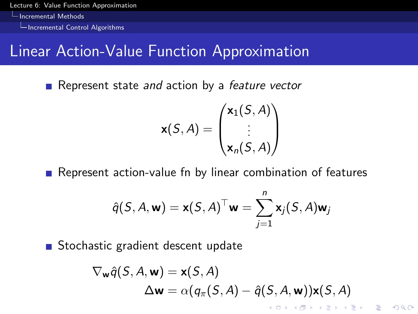
Lecture 6 Value Function Approximation, slide 23

Three slides of machinery you have already seen — the same derivation as p.12→16 with $q$ substituted for $v$ . Nothing new is claimed and nothing new happens.

The one structural change worth noticing: the features are now $x(S,A)$ , functions of both state and action. This is what permits generalization across actions as well as across states — or forbids it, if you use the common pattern of giving each action its own disjoint block of features via an indicator, as the chain walk example does on p.53. That choice is yours and the slides do not flag it as a choice.

p.25–26 · Mountain Car ⏱ 56:41

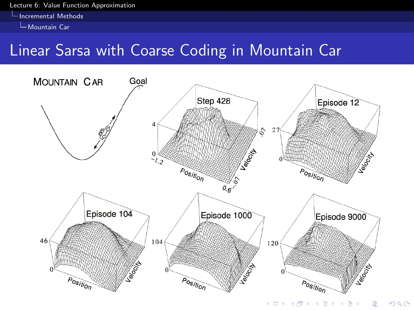
Lecture 6 Value Function Approximation, slide 25

An underpowered car in a valley. It cannot drive straight up, so it must reverse to build momentum — meaning the optimal action points away from the goal for part of the trajectory, which is why the problem is a standard benchmark rather than a toy.

State space is two-dimensional and continuous: position and velocity. The function approximator is coarse coding — many overlapping tiles of varying shape and size. Visiting a state pushes up every tile covering it and no others, so generalization is local and its radius is set by tile size.

Read the vertical axis before you read the shape

The surface grows across the panels — roughly $4 \to 27 \to 104 \to 120$ — while the policy is simultaneously getting better. That is impossible for a value function under this problem's $-1$ -per-step reward, where improvement should push values toward zero.
The axis is cost-to-go, $-\max_a\hat q(s,a,\mathbf{w})$ — confirmed against Sutton & Barto 2e Figure 10.1, which is the source of this figure and labels it exactly that way. The growth is the approximator progressively discovering how genuinely expensive the far states are, starting from a near-zero initialization.

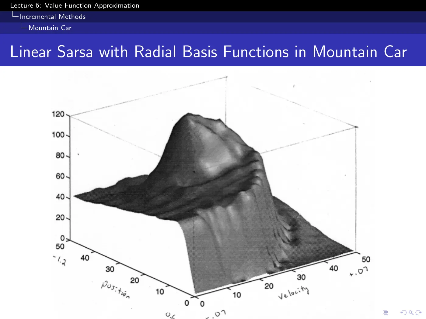
Lecture 6 Value Function Approximation, slide 26

The spiral is the converged approximation to the optimal value function, here with radial basis functions instead of tiles. It is smooth because the approximator interpolates — there is no exact value stored anywhere in it.

The state space is continuous. Is the action space continuous too, and what would change if it were?

Not here — the actions are discrete (accelerate forward, accelerate backward, or coast), and this is a bang-bang control problem: the optimum always sits at one extreme of the acceleration range, so intermediate values are never used.
With a continuous action space Sarsa still applies, but $\max_a\hat q(s,a)$ stops being a scan over a handful of outputs and becomes an optimization problem solved at every time-step. That cost is a standing objection to value-based control in continuous domains, and it is one of the motivations for L7's policy-based methods.

Could a better choice of state representation make this spiral simpler to learn?

Separate the underlying Markov state from the representation given to the learner. The physical variables and dynamics determine the value function, but you may choose coordinates and features — as long as the resulting representation retains the information needed for a Markov decision problem.
Good features can turn a difficult surface into one that is easy to approximate. They simplify the learning problem, not the underlying control problem.

p.27 · Study of λ — Should We Bootstrap? ⏱ 1:04:16

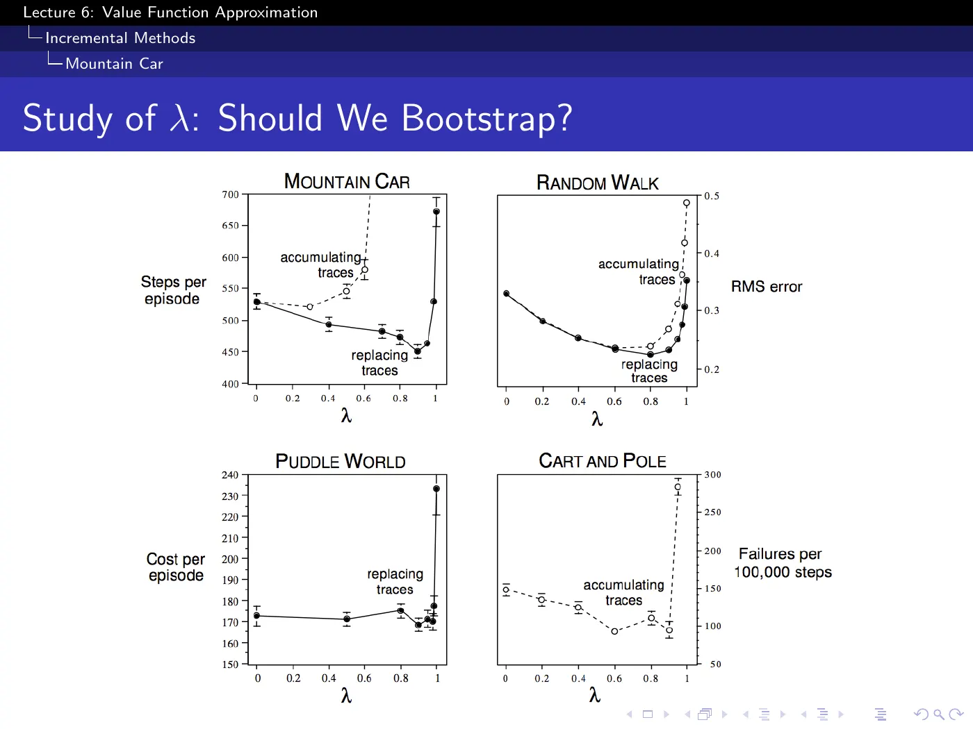
Lecture 6 Value Function Approximation, slide 27

Four domains, four different y-axis quantities — steps per episode, RMS error, cost per episode, failures per 100,000 steps — but all four are "lower is better", so all four curves tell the same story. Ignore the accumulating-versus-replacing distinction; those are two minor trace variants, not the point.

The point is the shape: $\lambda=1$ (pure MC) is bad everywhere, because of its variance. $\lambda=0$ is better. The optimum sits strictly between, and where it sits depends on the domain.

Why this slide is placed here and not in L4

It is the justification for the next four slides existing at all. Bootstrapping is not a stylistic preference — it wins empirically and consistently. If MC were competitive you would simply use MC and keep all the convergence guarantees, because MC never diverges anywhere in any table in this lecture.
The convergence problems from p.28 onward are the price of a benefit you have just been shown is real. That framing is what makes Gradient TD worth inventing rather than worth avoiding.

5 · When it breaks

p.28–29 · Baird's Counterexample ⏱ 1:05:47

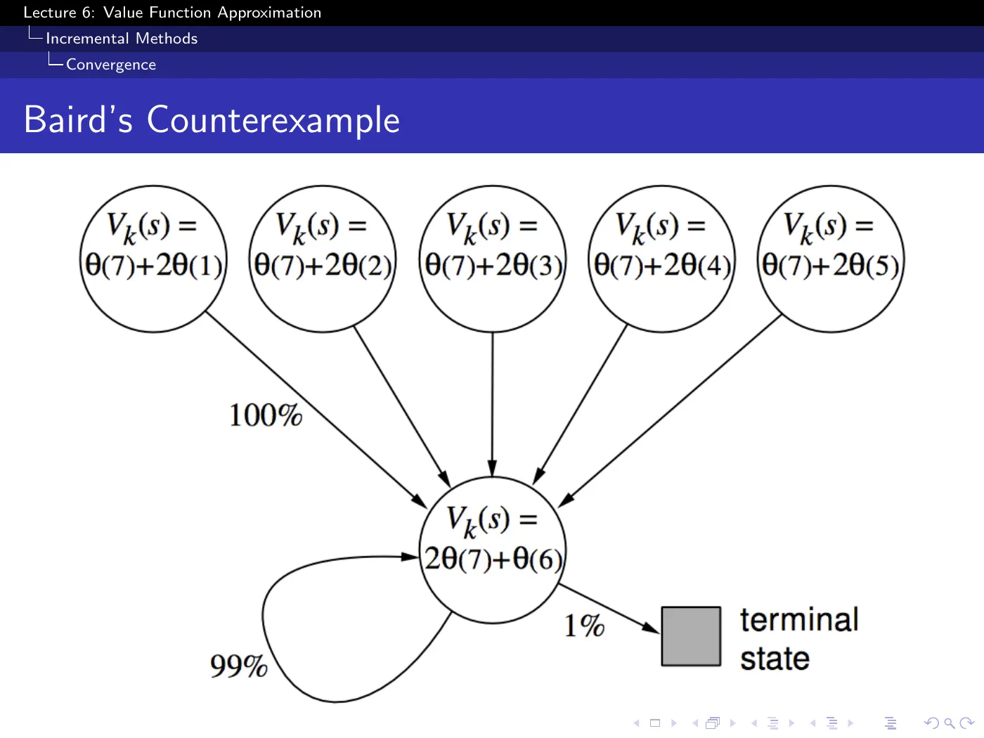
Lecture 6 Value Function Approximation, slide 28

Shown without explanation in the lecture. Filled in here from Sutton & Barto 2e §11.2, because the setup is what makes the result significant.

The construction. Seven states, two actions, $\gamma=0.99$ . The dashed action goes to one of the six upper states uniformly; the solid action goes to the seventh. Behaviour policy $b$ picks dashed with probability $6/7$ , so its next-state distribution is uniform. Target policy $\pi$ always takes solid, so the on-policy distribution for $\pi$ concentrates on state 7. The reward is zero on every transition.

Everything about this problem is as favorable as it could possibly be

$r\equiv 0$ , so the true value function is $v_\pi(s)=0$ everywhere — and it is exactly representable, by $\mathbf{w}=\mathbf{0}$ . There are 8 weights for 7 states, so solutions are not even unique, and the feature vectors are linearly independent.
Semi-gradient TD(0) diverges under the standard expected update from generic initializations; simply choosing a smaller positive step size does not repair the unstable direction. The example removes sampling noise and asynchrony, so the failure cannot be blamed on either. Nor can it be blamed on insufficient representational capacity, since the true value is representable.

Why off-policy is the ingredient that breaks it. On-policy, a transition into a high-valued state must eventually be followed by a transition out of it, and that exit correction is what keeps the estimates consistent: each state can support the one before it only by predicting a still-higher value later, and that prediction is eventually checked. Off-policy, you can take an action the target policy would never take, and the check never comes; the unverified prediction stands.

The counterexample combines three ingredients:

Bootstrapping — TD rather than MC.
Function approximation — here merely linear, with the value of each state written as an overlapping combination of shared parameters.
Off-policy updating — sweeping over all states uniformly rather than visiting them according to the policy being followed.

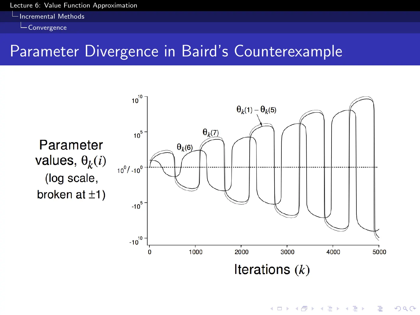
Lecture 6 Value Function Approximation, slide 29

This is not oscillation around a fixed point

The y-axis is logarithmic and broken at $\pm 1$ . The curves are not wobbling near zero; the parameters are growing by orders of magnitude while flipping sign. The MDP has seven states and linear features — this is as small as a counterexample gets, which is the point.

Later literature names this combination the deadly triad — Sutton & Barto's term (2e §11.3), not this 2015 lecture's. Treat it as a high-risk interaction, not as a theorem saying that every pair is safe. In particular, the lecture's own table allows on-policy TD with non-linear approximation to diverge even without the off-policy leg. In the linear case emphasized by Baird's example, switching to on-policy data or removing bootstrapping restores the standard convergence result.

The failure already appears in prediction, and even under an expected DP-style update. It is therefore not caused by GPI, exploration noise, or an unknown environment.

p.30 · Convergence of Prediction Algorithms ⏱ 1:06:32

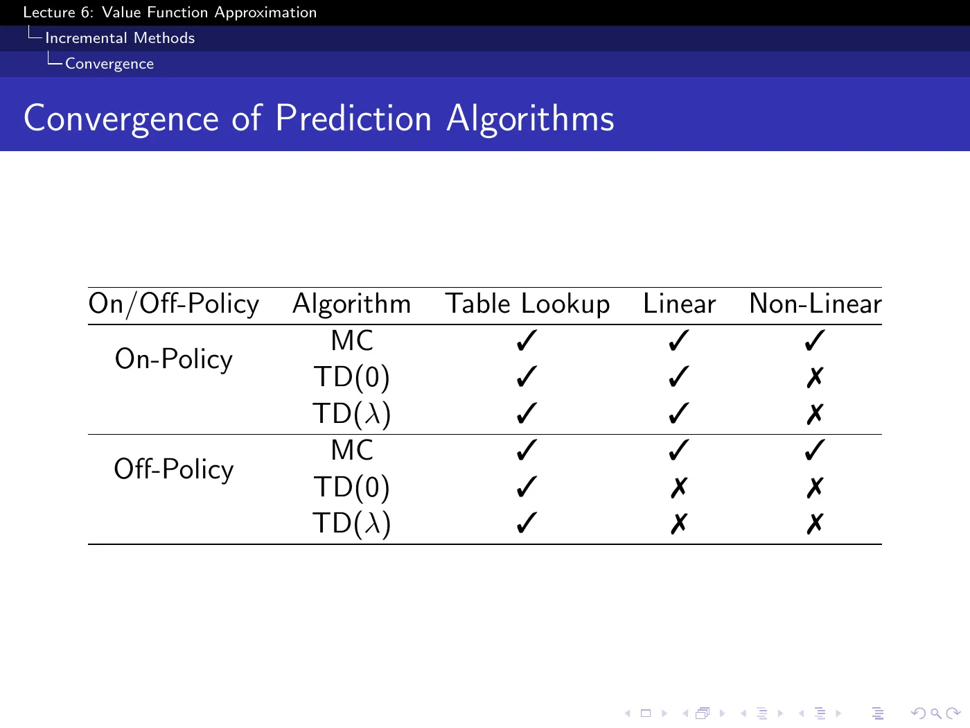
Lecture 6 Value Function Approximation, slide 30

Do not memorize twelve cells. Memorize the pattern:

The MC row is entirely ✓ under the table's assumptions. Its target does not depend on $\mathbf{w}$ (p.17), so it is true SGD on a fixed objective.
Every ✗ in the table is a TD entry. Every single failure in this lecture involves bootstrapping.
The table-lookup column is entirely ✓. That is L1–L5, and this is the retroactive explanation of why none of it ever misbehaved.
The table highlights two failure regions for ordinary TD: non-linear approximation can fail even on-policy, while off-policy learning can fail already in the linear case. This is a map of the lecture's guarantees, not an exhaustive taxonomy of every possible failure mechanism.

✓ does not mean "converges to the right answer"

It means the parameters reach a fixed point. Whether that fixed point is the one you want is a separate question with a separate answer: you land close to the best parameter vector representable by your approximator — not at the true $v_\pi$ , which is generally outside your representable set entirely.
Two distinct gaps are stacked here and the tick mark hides both: the gap from $v_\pi$ to the best representable approximation (due to the choice of features), and the gap from that to the TD fixed point (the algorithm's, and $\gamma$ -dependent — p.18).

p.31 · Gradient Temporal-Difference Learning ⏱ 1:08:06

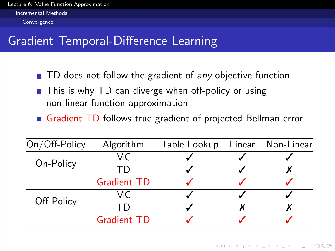
Lecture 6 Value Function Approximation, slide 31

The first bullet is the most important sentence in the lecture:

"TD does not follow the gradient of any objective function."

Not merely "TD's squared-error objective is hard to optimize." The ordinary semi-gradient update is not generally the gradient of one fixed scalar prediction objective, so the usual argument that every expected step descends a loss is unavailable. Special cases can admit alternative interpretations, but the generic update field need not be conservative. This is the direct consequence of the semi-gradient at p.18: ignoring the target derivative preserves a practical fixed-point update but gives up the ordinary regression guarantee.

Gradient TD repairs the basic problem by constructing an explicit objective — typically the mean-squared projected Bellman error — and following its gradient with an auxiliary correction estimate. The slide marks Gradient TD as convergent across its table, including the non-linear column. Read that as the lecture's high-level map: exact guarantees depend on the particular Gradient-TD algorithm, assumptions, and function class. Emphatic TD is mentioned as another stability-oriented approach, without a derivation.

p.32 · Convergence of Control Algorithms ⏱ 1:08:52

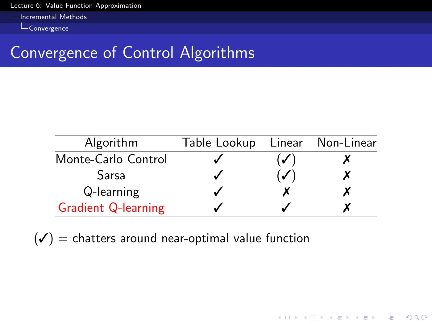
Lecture 6 Value Function Approximation, slide 32

Control is worse than prediction, and it fails for a different reason, which the slide does not give.

In prediction the problem is the bootstrap target. In control there is a second, independent failure: the policy improvement step is no longer guaranteed to improve the policy. The $\epsilon$ -greedy improvement theorem of L5 assumed you held $q_\pi$ exactly; with an approximation, acting greedily with respect to $\hat q_\mathbf{w}$ can produce a genuinely worse policy. Repeated evaluation and improvement can therefore chatter among policies instead of settling.

Read the two failure modes as different symbols:

Symbol	Meaning	Severity
(✓)	may chatter within a bounded region near the optimum	usually acceptable
✗	catastrophic divergence is possible	serious

Q-learning is ✗ even with linear approximation, where Sarsa is (✓) — the penalty for being off-policy, exactly as in the prediction table.

Theory versus practice, stated plainly in the lecture

Where divergence actually bites is neural networks. Apply naive Q-learning or Sarsa to one and it very often diverges: steep regions produce large gradients, a large step swings the policy, the policy change reshapes the value function, and the process spirals.
With linear approximation, even off-policy where the table says ✗, it mostly works in practice — you have to try fairly hard to break it. The ✗ marks possibility, not frequency.
Keep this asymmetry in mind, because the next section builds a system that lands squarely in the worst cell of this table and makes it work anyway.

6 · Batch methods

p.34–35 · Batch Reinforcement Learning ⏱ 1:11:57

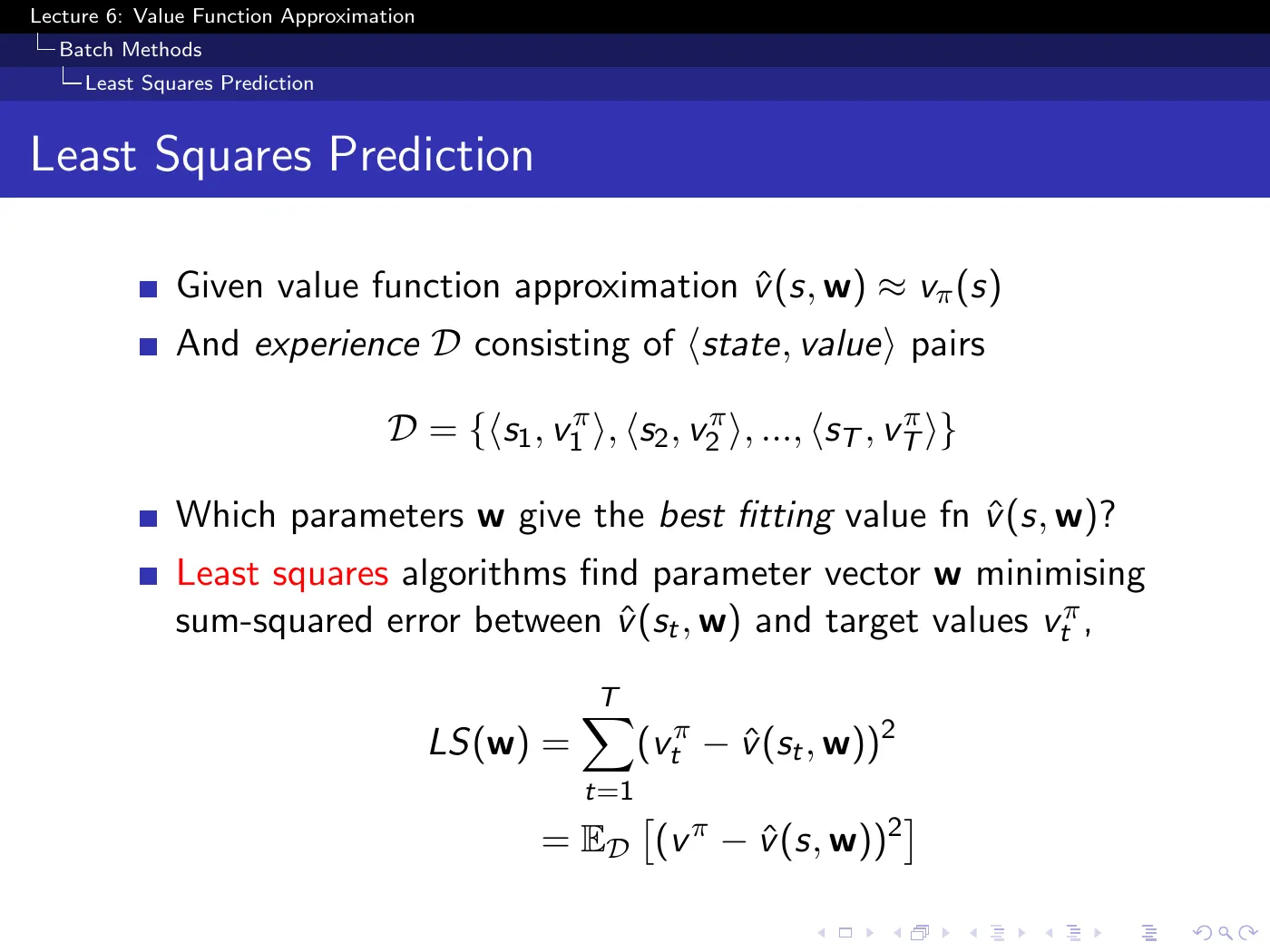
Lecture 6 Value Function Approximation, slide 35

LS(\mathbf{w})=\sum_{t=1}^{T}\big(v_t^\pi-\hat v(s_t,\mathbf{w})\big)^2=\mathbb{E}_\mathcal{D}\big[(v^\pi-\hat v(s,\mathbf{w}))^2\big]

The complaint against everything in the first half: you see a transition once, take one small step, and throw the data away. That is fine when experience is free and wasteful when it is not — a robot's experience costs wall-clock time and hardware wear.

Note the oracle is back. The pretend-then-substitute cycle is starting for the third time, and p.44 will replace this oracle exactly as p.16 replaced the first one.

p.36–37 · Stochastic Gradient Descent with Experience Replay ⏱ 1:15:00

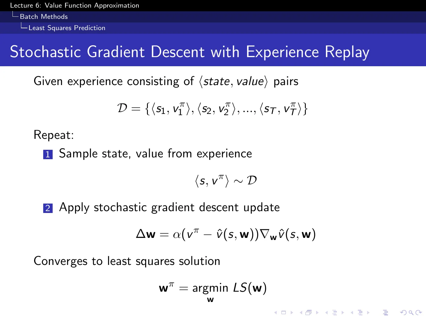
Lecture 6 Value Function Approximation, slide 37

Experience replay is not a new algorithm

It is the same SGD update from p.12, applied repeatedly to a stored dataset in random order. Nothing about the learning rule changes. What changes is what you feed it and in what sequence.

It buys two things, and only the first is obvious:

Sample efficiency — each transition is reused many times, so you extract more from data you have already paid for. For a fixed supervised objective and suitable optimization conditions, repeated SGD can approach that objective's empirical-risk minimum; this is not a blanket guarantee for bootstrapped RL.
Decorrelation — sampling uniformly at random from the buffer destroys the trajectory ordering. This is a direct answer to the non-i.i.d. half of p.9, and it is the reason replay stabilizes neural networks rather than merely making them cheaper to train.

7 · DQN

p.38 · Experience Replay in Deep Q-Networks ⏱ 1:17:16

Lecture 6 Value Function Approximation, slide 38

\mathcal{L}_i(w_i)=\mathbb{E}_{s,a,r,s'\sim\mathcal{D}_i}\left[\Big(r+\gamma\max_{a'}Q(s',a';\,\underbrace{w_i^-}_{\text{old, frozen}})-Q(s,a;\,\underbrace{w_i}_{\text{current}})\Big)^2\right]

DQN is the impossible cell of p.32, made to work

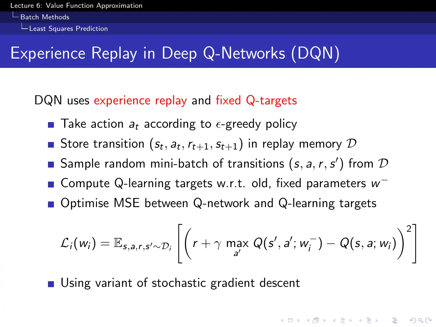
Off-policy Q-learning + bootstrapping + non-linear approximation occupies the most unstable corner of the control table — all three legs of the deadly triad at once. Replay and target networks made that combination work empirically at Atari scale; they reduce two major pathologies but do not turn the method into a generally convergent algorithm.

Trick 1 — experience replay breaks the correlation between consecutive updates (non-i.i.d.).

Trick 2 — fixed Q-targets breaks the coupling between the prediction and the thing it is chasing (non-stationarity). The two $w$ symbols in the loss are different parameter vectors, and missing that is missing the entire slide. If they were the same, every update would move the target as well as the prediction, and with a non-linear approximator that feedback loop is what spirals out of control.

Freezing $w^-$ makes the target locally more stationary with respect to the network parameters. The replay buffer and its sampling distribution may still change, so this is not a fully stationary supervised-learning problem. Every few thousand steps, $w^-\leftarrow w$ and the next phase begins. The swap interval is a tuned hyperparameter; smoothly tracking variants are also possible. Silver relates this separation to fitted Q-iteration.

p.39 · DQN in Atari ⏱ 1:24:07

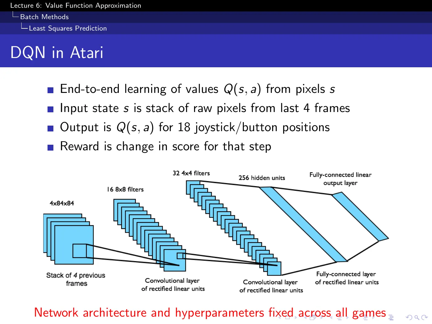
Lecture 6 Value Function Approximation, slide 39

The architecture is the action-out design from p.7 — 18 Q-values from a single forward pass, which is what keeps $\arg\max_a$ affordable at every frame.

Why the input is four frames rather than one

A single Atari frame is not a Markov state. From one image you cannot tell which way the ball is moving. Stacking the last four frames restores enough information to make velocity observable, and only then is the MDP formulation the whole course rests on actually legitimate.
This is a state-construction decision, not a network-architecture decision, and it is the kind of thing that silently invalidates everything upstream when you get it wrong. The slide lists it as an implementation detail.

p.40–41 · Results and Ablation ⏱ 1:24:52

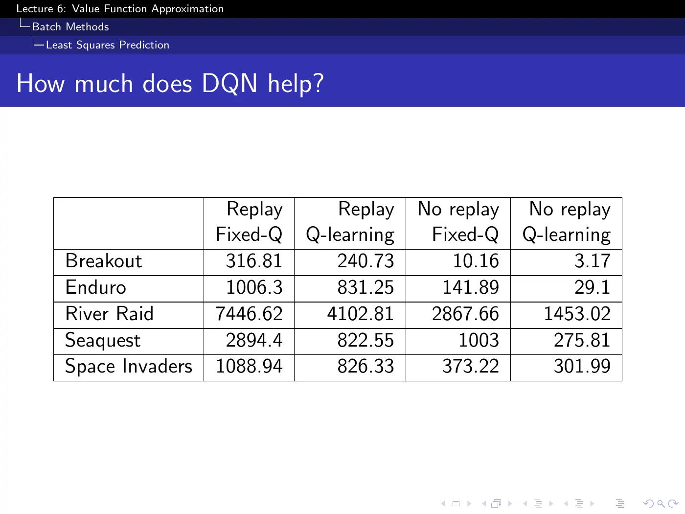
Lecture 6 Value Function Approximation, slide 41

The ablation is a $2\times 2$ : {replay, no replay} × {fixed-Q, plain Q-learning}. Both ideas help and they compose, but they do not help equally — replay is the dominant factor by a wide margin. On Breakout, removing replay collapses the score from 316.81 to 10.16 (a factor of ~31), while removing fixed-Q alone costs about 24%. The same ordering holds across all five games.

On p.40 the games are sorted by performance relative to an expert human tester. The tail matters more than the head:

Montezuma's Revenge marks the limit of this entire lecture

It scores near zero. The failure is not representational — the network is identical to the one winning at Video Pinball. It needs long sequences of correct actions before any reward appears, and $\epsilon$ -greedy exploration has no mechanism for that: random perturbation of a policy cannot stumble onto a hundred-step plan.
Nothing in L6 addresses this, because L6 is about representing value functions, not about finding the experience worth representing. That is L9.

8 · Closed-form least squares

p.42–43 · Linear Least Squares Prediction ⏱ 1:26:25

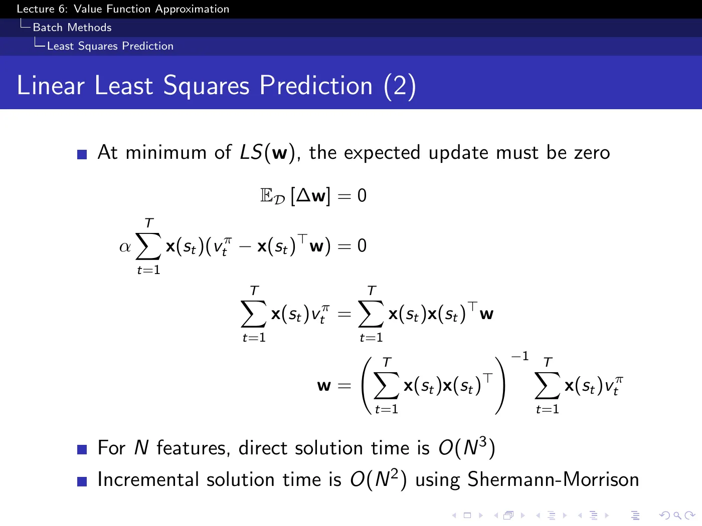
Lecture 6 Value Function Approximation, slide 43

\mathbb{E}_\mathcal{D}[\Delta\mathbf{w}]=0 \quad\Longrightarrow\quad \mathbf{w}=\left(\sum_{t=1}^{T}x(s_t)x(s_t)^\top\right)^{-1}\sum_{t=1}^{T}x(s_t)v_t^\pi

The derivation runs on one idea: at the least-squares minimum you would no longer choose to change $\mathbf{w}$ , so set the total update to zero and solve. Everything after that is collecting terms and observing that only one of them contains $\mathbf{w}$ .

Two details the slide passes over:

$\alpha$ cancels. It multiplies the entire expression, which you are setting to zero, so the step size is irrelevant to the answer. There is no learning rate to tune here at all — that is a real practical advantage, not a curiosity.
$N$ is the number of features, not the number of states. $O(N^3)$ for the direct solve and $O(N^2)$ incrementally via Sherman-Morrison. Matrix inversion has been avoided throughout the course because it scaled with $|\mathcal{S}|$ ; here it does not, which is the only reason this section can exist.

The trade-off against experience replay is genuine and situational: few features with a long experience history favors the closed form; many features favors replay, and in practice five or six passes over the data already extract most of what is there.

p.44–46 · LSMC, LSTD, and LSTD(λ) ⏱ 1:31:45

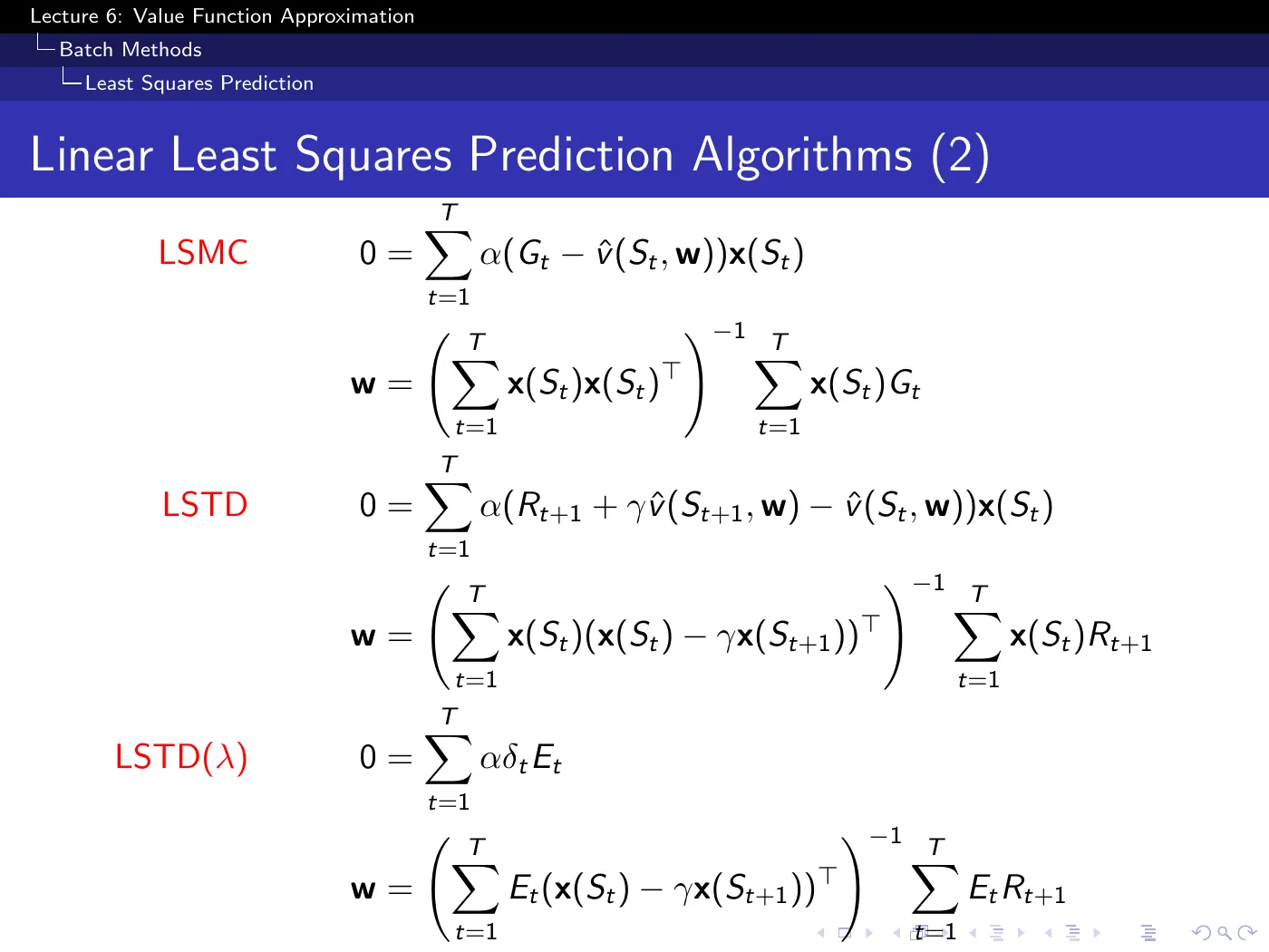
Lecture 6 Value Function Approximation, slide 45

The oracle assumed on p.35 is replaced by the same substitution as p.16 — $v_t^\pi\approx G_t$ , or $R_{t+1}+\gamma\hat v(S_{t+1},\mathbf{w})$ , or $G_t^\lambda$ .

The asymmetry of the LSTD matrix is bootstrapping made visible

LSMC inverts $\sum_t x(S_t)x(S_t)^\top$ — an outer product, symmetric, the ordinary least-squares design matrix.
LSTD inverts $\sum_t x(S_t)\big(x(S_t)-\gamma x(S_{t+1})\big)^\top$ — not symmetric, because the target reaches forward to the next state's features.
That broken symmetry is the algebraic trace of bootstrapping. It is the same asymmetry that, in the incremental setting, means the update is not the gradient of anything (p.31) — here it surfaces as a matrix that is not a covariance.

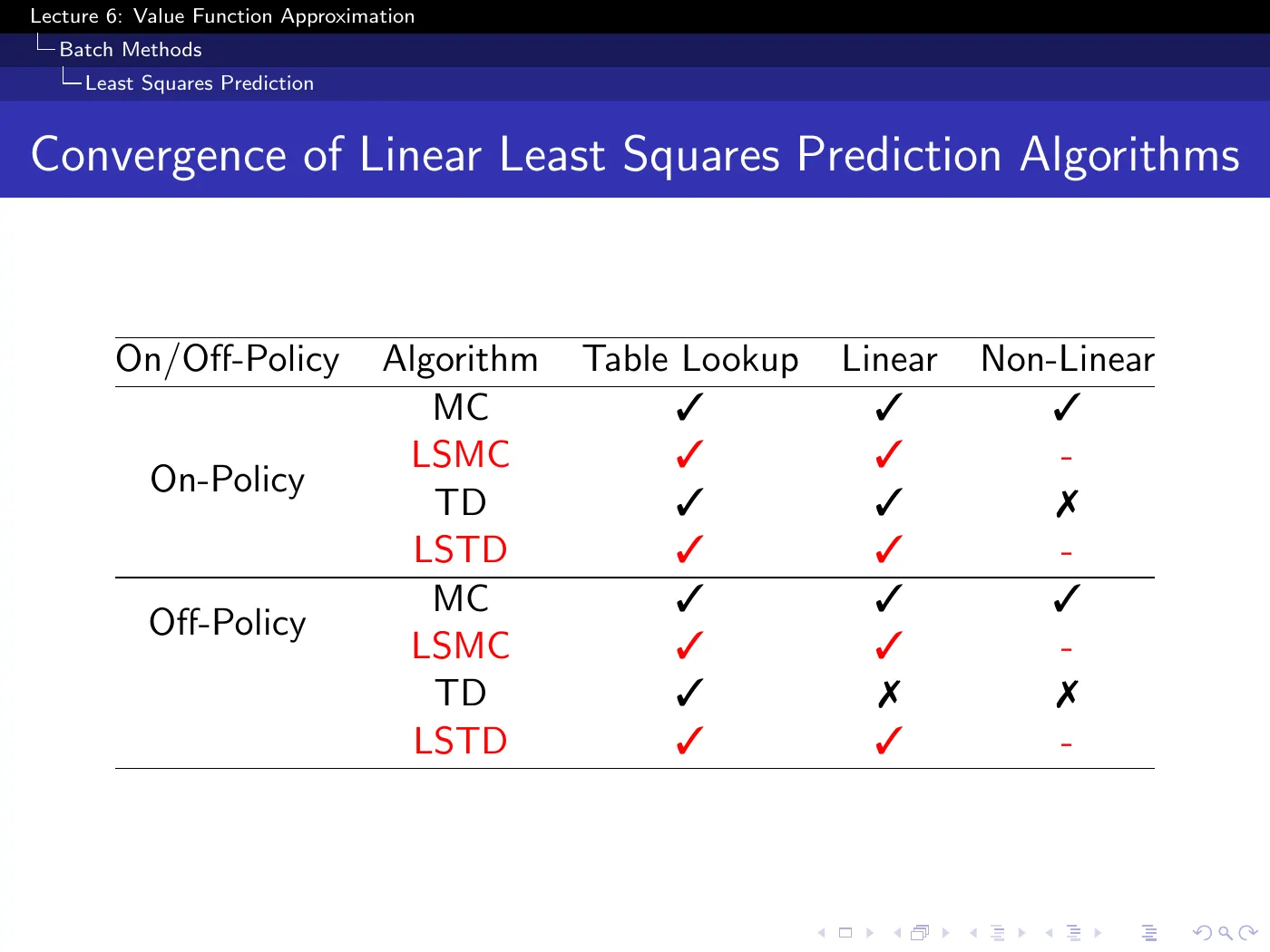
Lecture 6 Value Function Approximation, slide 46

The key row in the lecture's table is off-policy linear LSTD: ✓, where incremental linear TD is ✗. The point is that LSTD solves a linear fixed-point system from the batch instead of repeatedly applying the unstable incremental update. The tick still presumes adequate data coverage and a well-defined, nonsingular system; it is not a guarantee for every arbitrary off-policy dataset. The "-" entries under Non-Linear mean not applicable — the displayed closed form is exactly what linearity buys.

p.47 and p.52 · Least Squares Policy Iteration ⏱ 1:32:32

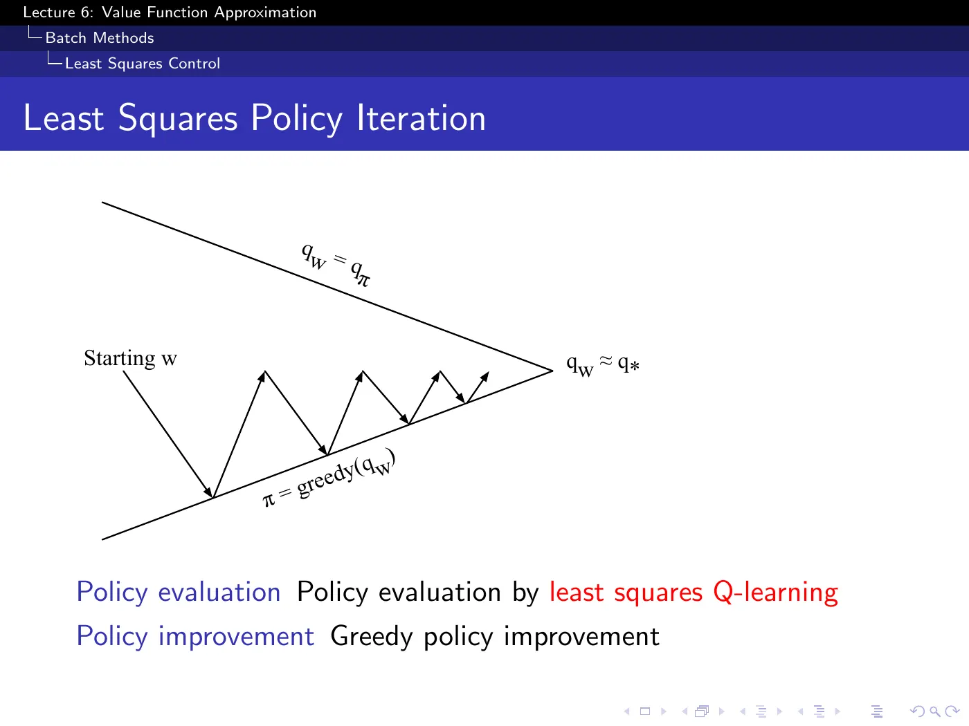
Lecture 6 Value Function Approximation, slide 47

GPI once more, with LSTDQ in the evaluation slot. One detail differs from p.21 and it is worth pausing on:

The improvement step is greedy here, not ε-greedy

On p.21 exploration had to be part of the improvement step, because the policy you improve to is the policy that generates your next data. In LSPI the batch $\mathcal{D}$ is fixed and collected in advance — the chain walk example uses 10,000 steps of a random walk and never gathers more. Exploration is therefore decoupled from improvement, and the improvement step can be purely greedy.
The cost is that each evaluation is generally off-policy, since the fixed batch came from a behavior policy that differs from the policy currently being evaluated. Linear LSTD can solve the corresponding batch fixed-point equations under coverage and nonsingularity conditions (p.46); the skipped slides p.49–50 provide the lecture's high-level justification.

LSPI still lacks a general guarantee of exact convergence to the optimal policy. On p.52 it joins Monte-Carlo control and Sarsa at (✓): approximate policy iteration can remain in a bounded neighborhood or cycle among policies. Solving the evaluation equations removes one source of error, but it does not restore the exact policy-improvement theorem lost under approximation (p.32).

p.53–55 · Chain Walk ⏱ 1:34:10

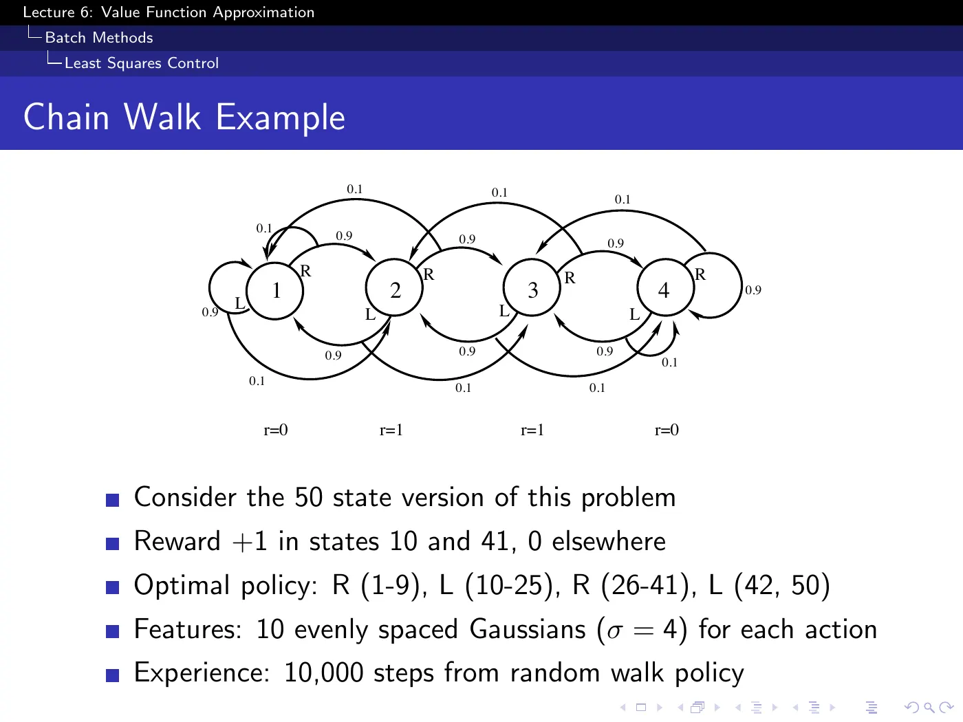
Lecture 6 Value Function Approximation, slide 53

50 states in a line, reward $+1$ at states 10 and 41 only, 10 evenly spaced Gaussians per action, and one fixed batch of 10,000 steps from a random walk policy.

The optimal policy is "head toward whichever reward state is nearer" — R for 1–9, L for 10–25, R for 26–41, L for 42–50. Reading it that way makes it memorable; reading it as four arbitrary intervals does not.

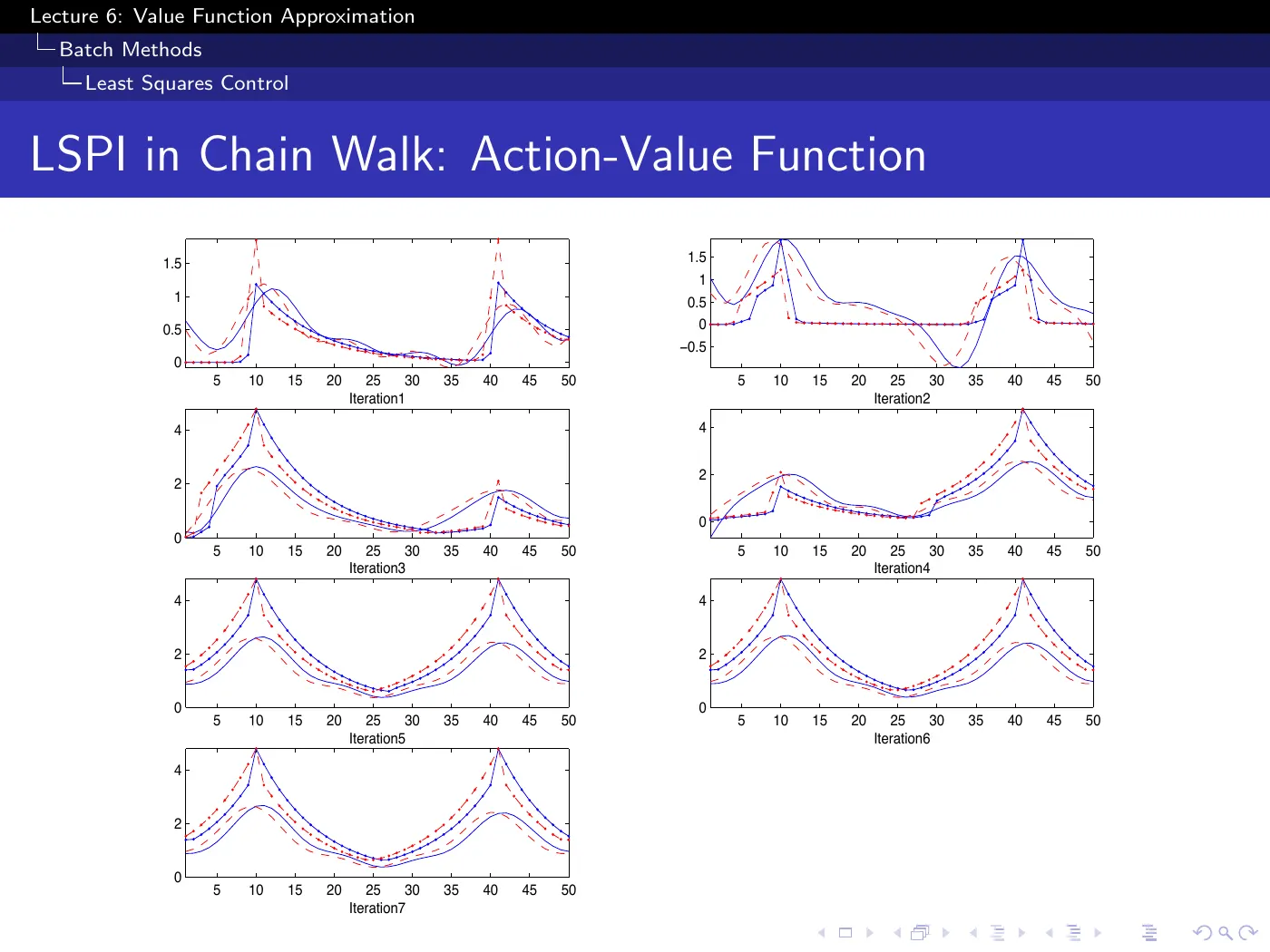
Lecture 6 Value Function Approximation, slide 54

Solid lines are the LSPI approximation, dashed are exact; blue and red are the two actions. The same 10,000 transitions are re-evaluated at every iteration — no new experience is ever collected. That is the entire demonstration: seven policy iterations, all obtained from one fixed batch, which is what "sample efficient" means concretely.

The peaks are broad rather than sharp for two independent reasons that are easy to conflate: value genuinely spreads along the chain through discounting, and the RBF approximator smooths on top of that. Only the second is an artifact.

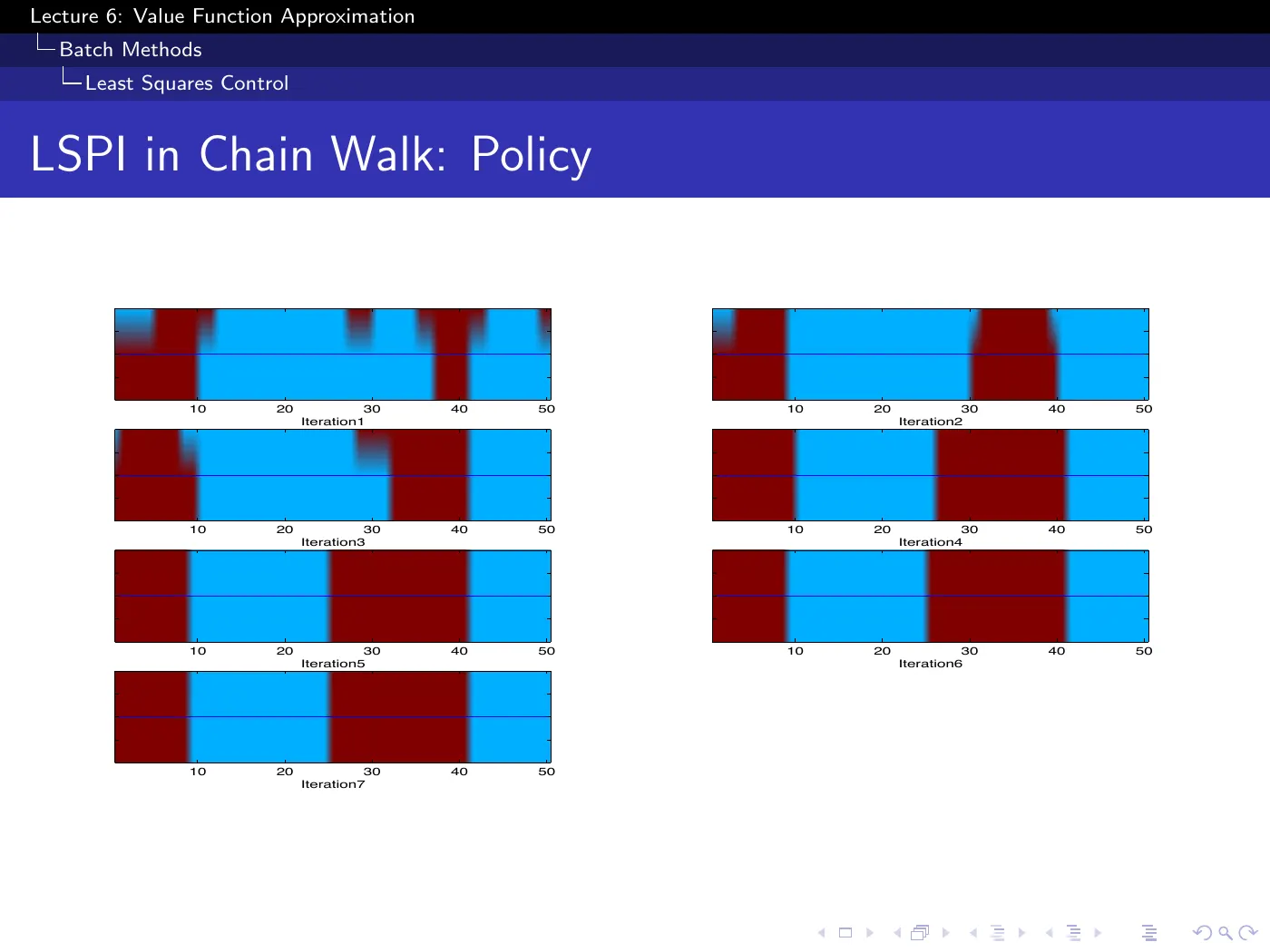
Lecture 6 Value Function Approximation, slide 55

The policy plots converge by iteration 7, and the decisions are right somewhat earlier than the value function looks converged — the $\arg\max$ only needs the ordering to be correct, not the magnitudes.

Study checklist

Close the note and answer these in your own words. Reopen only the section linked after the question.

Why is generalization more important than memory compression? → 1 · Why approximate at all
What does “linear” mean in $\hat v(s,\mathbf w)=x(s)^\top\mathbf w$ , and how does one-hot encoding recover a table? → 2 · The oracle assumption
Write the shared update template and the MC, TD(0), and TD( $\lambda$ ) targets. → 3 · Removing the oracle — prediction
Why is MC genuine SGD while ordinary TD is a semi-gradient method? → p.18 · TD Learning with Value Function Approximation ⏱ 37:24
How do Sarsa and Q-learning change when $Q$ becomes $\hat q(s,a,\mathbf w)$ ? → 4 · Control
Why can approximate policy improvement chatter even when prediction is stable? → p.32 · Convergence of Control Algorithms ⏱ 1:08:52
What does the deadly triad warn about, and why is it not an if-and-only-if theorem? → p.28–29 · Baird's Counterexample ⏱ 1:05:47
Why keep bootstrapping despite its stability risk? → p.27 · Study of λ — Should We Bootstrap? ⏱ 1:04:16
What problems do experience replay and a target network reduce, and what do they not guarantee? → 7 · DQN
Distinguish LSMC, LSTD, LSTD( $\lambda$ ), and LSPI by target and role. → 8 · Closed-form least squares

Gaps to close on your own

Slides p.48–51 are left as a reading exercise

The lecture ran short and skipped straight from LSPI's diagram to the chain walk example, explicitly deferring four slides. They contain the argument for why least-squares control must be off-policy, and the actual LSTDQ derivation.

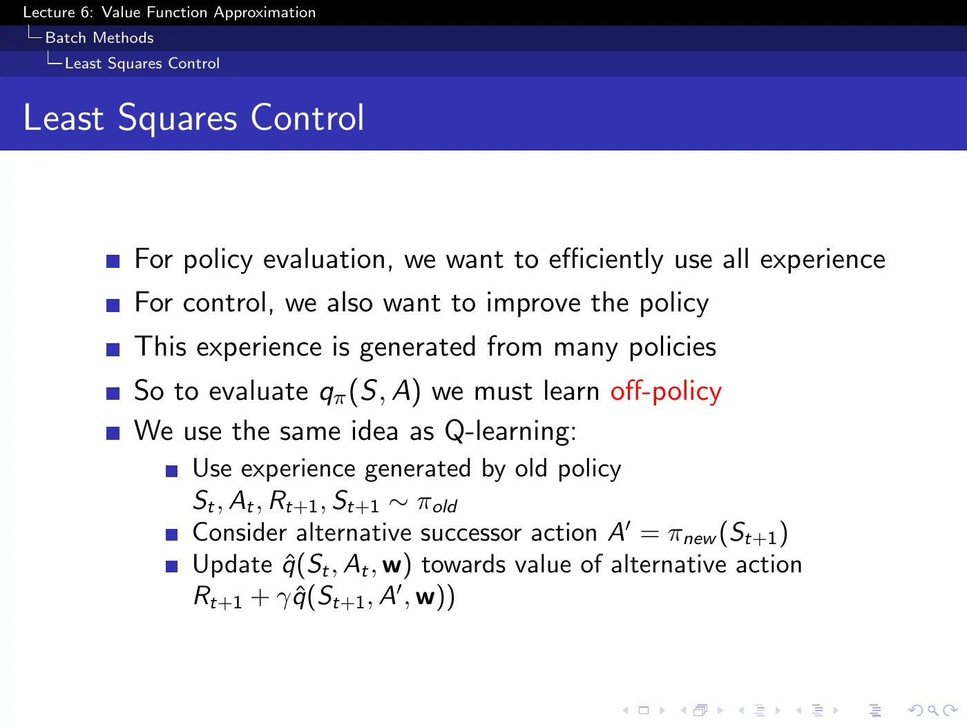
Lecture 6 Value Function Approximation, slide 49

This is the slide that justifies the greedy improvement step on p.47 — experience is generated from many policies, so evaluating $q_\pi$ for the current one is necessarily off-policy, and the fix is Q-learning's: take $S_t,A_t,R_{t+1},S_{t+1}\sim\pi_\text{old}$ from the batch, but bootstrap toward the action $A'=\pi_\text{new}(S_{t+1})$ that the new policy would take.

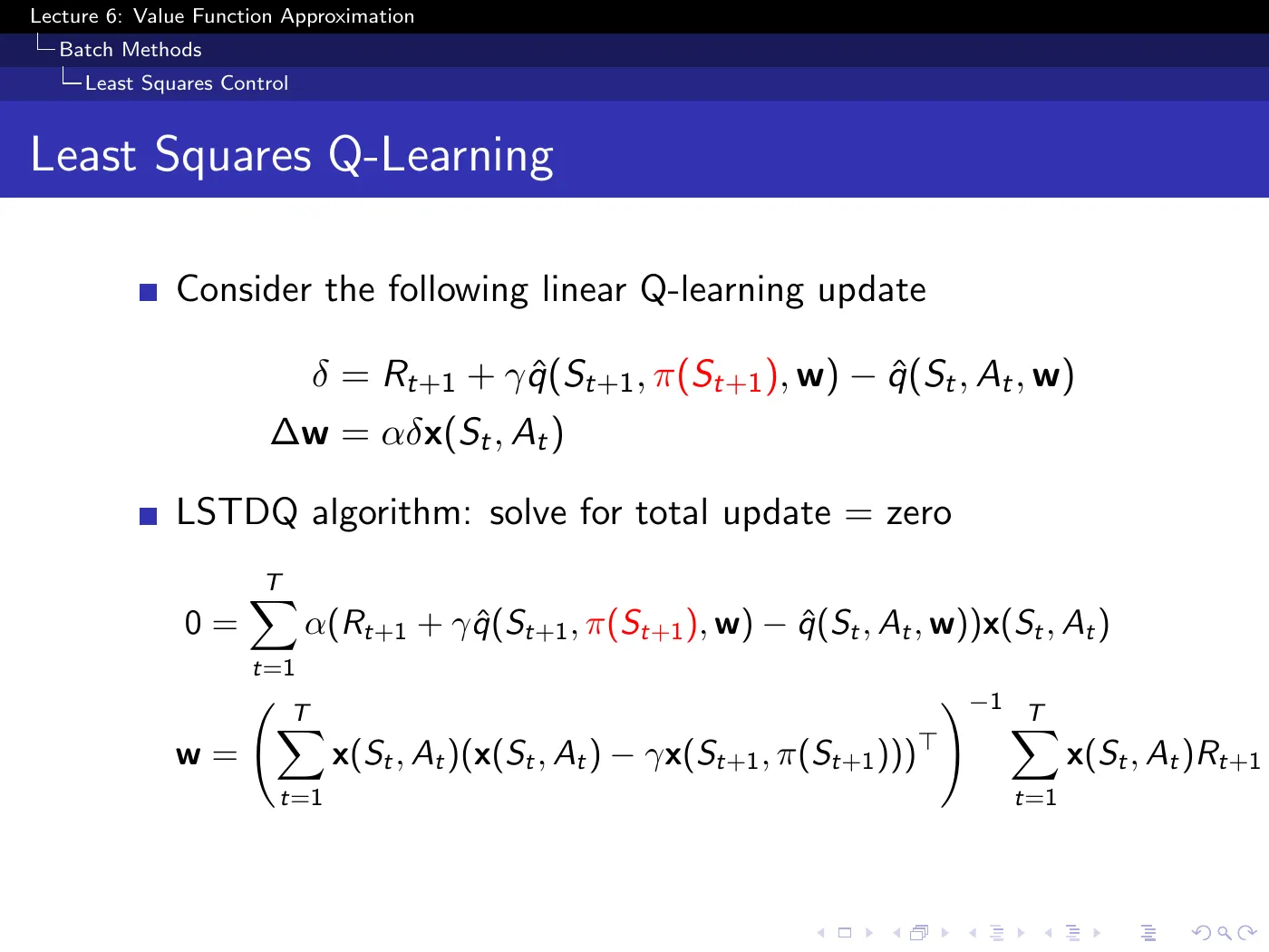
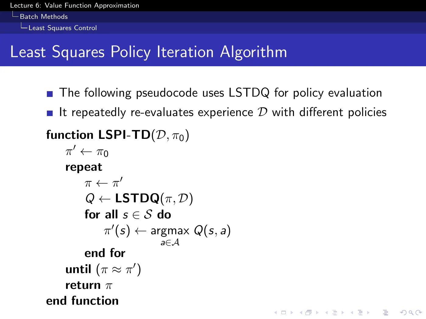
Lecture 6 Value Function Approximation, slide 50

Lecture 6 Value Function Approximation, slide 51

Work through p.50's LSTDQ solution and p.51's pseudocode together — the pseudocode makes clear that the same $\mathcal{D}$ is passed to LSTDQ on every iteration, which is the point of the whole algorithm.

DQN reward clipping. The slide says "reward is change in score for that step" and separately that one hyperparameter set covers all 50 games. Those two claims sit uneasily together, since raw score deltas differ by orders of magnitude across games. Check the Nature paper for how rewards were normalized — it is not mentioned in this lecture.
Gradient TD and emphatic TD. Named and credited with fixing everything, with no derivation of the projected Bellman error or the correction term. If you intend to work off-policy with non-linear approximation, this is the gap that matters most — Sutton & Barto 2e Ch. 11 is the treatment, and §11.3's argument about which leg of the triad to give up is the part worth reading first.
Feature discovery. Explicitly out of scope: the lecture assumes someone hands you good features. The answer it points to is "use a neural network," which is what makes L6's non-linear column the one modern work actually lives in.

Language notes

Phrasings worth borrowing for your own technical writing and talks:

Expression	Use
something's got to give	the current approach cannot survive the next constraint
squeeze more juice out of the data	extract additional value from a fixed sample
we've cheated	flagging an assumption you are about to pay back
think of this as a copy-and-paste exercise	signalling that a derivation is structurally identical to a previous one
you don't want to reverse the flow of time	rejecting a symmetric update where asymmetry is load-bearing
it chatters around the optimum	oscillating in a bounded region without converging
you have to work a bit harder to break the algorithm	failure is possible in theory but rare in practice
I wouldn't claim this is the most aesthetically satisfying idea, but in practice it stabilizes everything	defending an inelegant fix on empirical grounds
a standing objection to	a known, unresolved criticism of an approach
the honest limit of	naming what a method genuinely cannot do