Silver RL·Lecture 3·Lecture Notes
Lecture 3 · Planning by Dynamic Programming
Slides: David Silver, UCL Course on Reinforcement Learning (2015), CC BY-NC 4.0. Some slide content is from third parties and is outside that licence.
Slides: David Silver - RL Course (UCL 2015) · Previous: Lecture 2 · Markov Decision Processes · Next: Lecture 4 · Model-Free Prediction
Companion: Silver RL Lecture 3 — Question List (your own stuck points, in Korean) · Contraction Mapping & Bellman Convergence
Read this instead of watching. Each slide is embedded below with only what the slide itself does not say — the reasoning, the caveats, and the questions worth being able to answer.
The one idea
L2 wrote down the Bellman equations and left them as equations. L3 does one thing to them:
Turn the equality into an assignment, and iterate.
Everything else follows from which Bellman equation you iterate. Slide p.26 is the entire lecture in one table:
| Problem | Bellman equation | Algorithm |
|---|---|---|
| Prediction | expectation | iterative policy evaluation |
| Control | expectation + greedy improvement | policy iteration |
| Control | optimality | value iteration |
DP needs two properties, and the MDP supplies each from a different object:
- Optimal substructure — the problem decomposes into subproblems. This is the Bellman equation: the value of a state is one step plus the value of the successor.
- Overlapping subproblems — the same subproblem recurs, so answers can be cached. This is the value function: a store of "how much reward can I get from here onward", computed once and reused everywhere it appears.
That reframing is worth keeping: the value function is a cache. Every algorithm in this course is a scheme for filling it in.
Somebody hands you and — the full source code of the environment. Nothing here works without them, which is exactly the assumption L4 removes.
Keep the two axes separate, because the course is organized by them: planning vs learning (do you know the model?) and prediction vs control (evaluate a given policy, or find the best one?). L3 is planning; both halves of the second axis appear here.
Contents
- 1 · What dynamic programming is
- 2 · Iterative policy evaluation
- 3 · Policy iteration
- 4 · Why greedy improvement works
- 5 · How much evaluation is enough
- 6 · Value iteration
- 7 · The summary, and complexity
- 8 · Asynchronous dynamic programming
- 9 · The bridge to model-free RL
- Study checklist
- Gaps to close on your own
- Language notes
1 · What dynamic programming is
p.3–6 · Requirements and Scope ⏱ 2:18
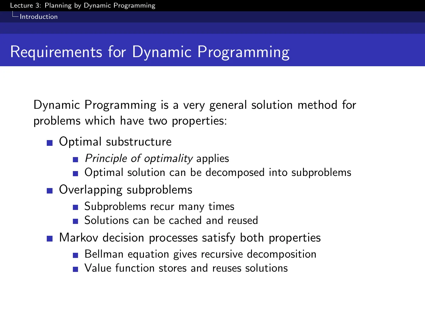
Neither word means what it looks like. Dynamic = the problem has a sequential or temporal structure. Programming = mathematical programming, as in linear programming — optimizing a "program", which for mathematicians means what we call a policy. Nothing to do with writing code.
The shortest-path example makes both DP properties concrete at once: the shortest path from here to the wall decomposes through a midpoint (optimal substructure), and the sub-path from that midpoint gets reused by many different starting points (overlapping subproblems).
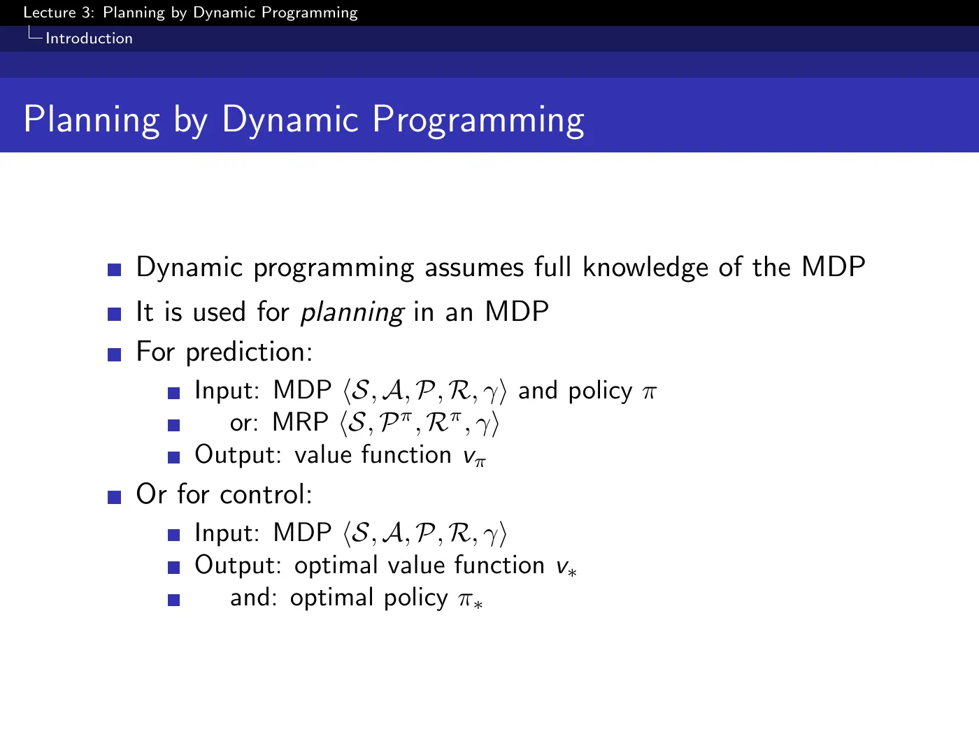
The two planning problems, and note that the second contains the first:
- Prediction: given MDP + policy → . Equivalently, flatten the MDP under into an MRP and evaluate that.
- Control: given MDP → , and hence .
DP is far older and broader than RL — scheduling, sequence alignment, shortest paths, the Viterbi algorithm. What is special here is only that the Bellman equation supplies the recursion.
2 · Iterative policy evaluation
p.7–8 · The Update ⏱ 12:56
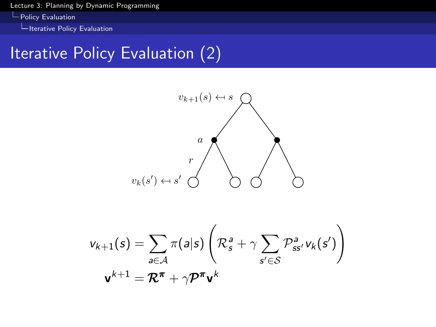
Read the backup diagram as every state taking a turn at being the root. One sweep = each state gets one one-step lookahead, using the previous iteration's values at the leaves.
Synchronous means the whole new value function is computed from the whole old one before anything is swapped in. That is a choice, not a requirement — p.29 drops it.
The starting point is arbitrary; zeros everywhere is the natural choice and means "I expect no reward anywhere."
Two distinct questions are open at this point: does a value function satisfying the equation exist and is it unique, and does this iteration reach it. Both are answered by the contraction mapping theorem on p.35–42 — which the lecture ran out of time for → Contraction Mapping & Bellman Convergence.
p.9–11 · Small Gridworld ⏱ 19:45
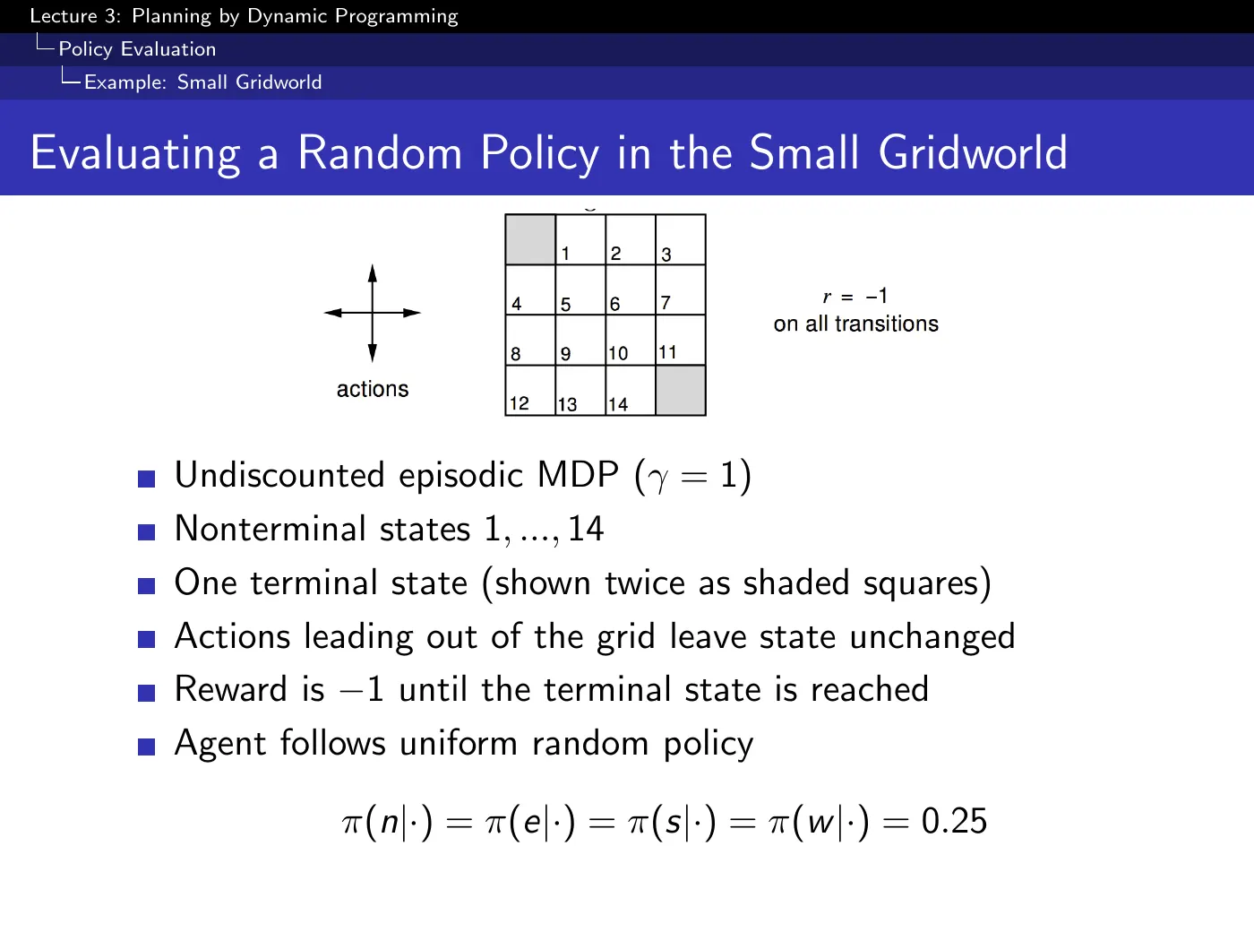
grid, two terminal corners, per step, uniform random policy, . Since every step costs exactly , the value of a state is minus the expected number of steps to termination — the question "how good is this state?" and "how long until I get out?" are the same question.
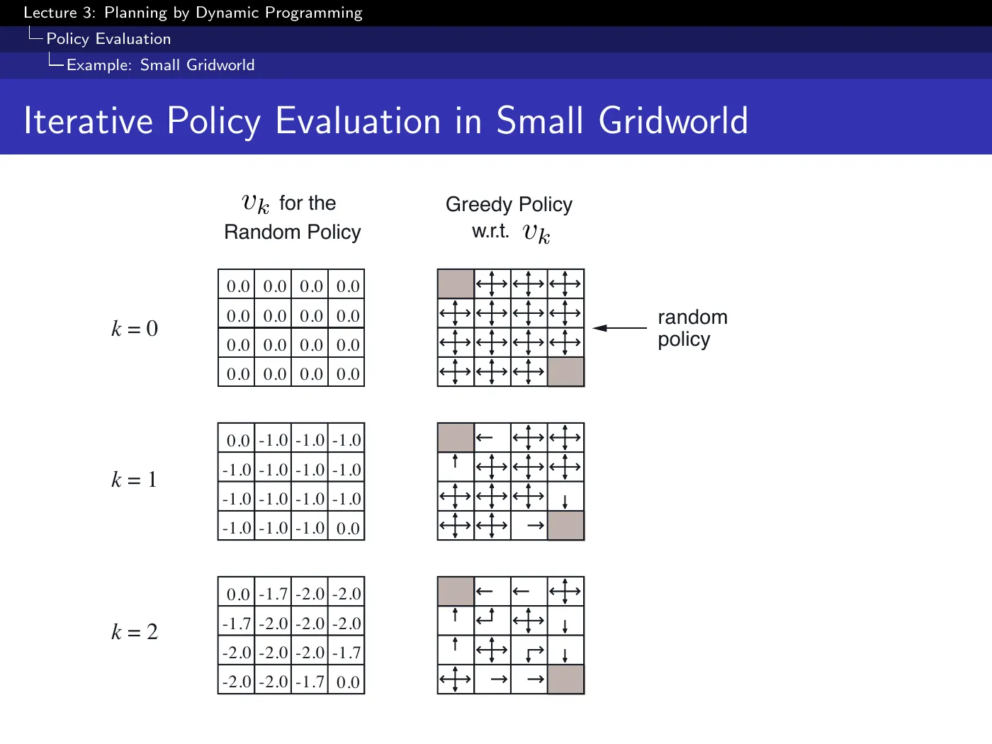
Work one cell by hand and the mechanism becomes concrete. At , a cell adjacent to the terminal corner: three directions give , and the one leading to the terminal gives . Average over the four with probability each:
which the slide prints as — it is truncated to fit, not rounded to something else. Several cells that look identical differ past the displayed decimal.
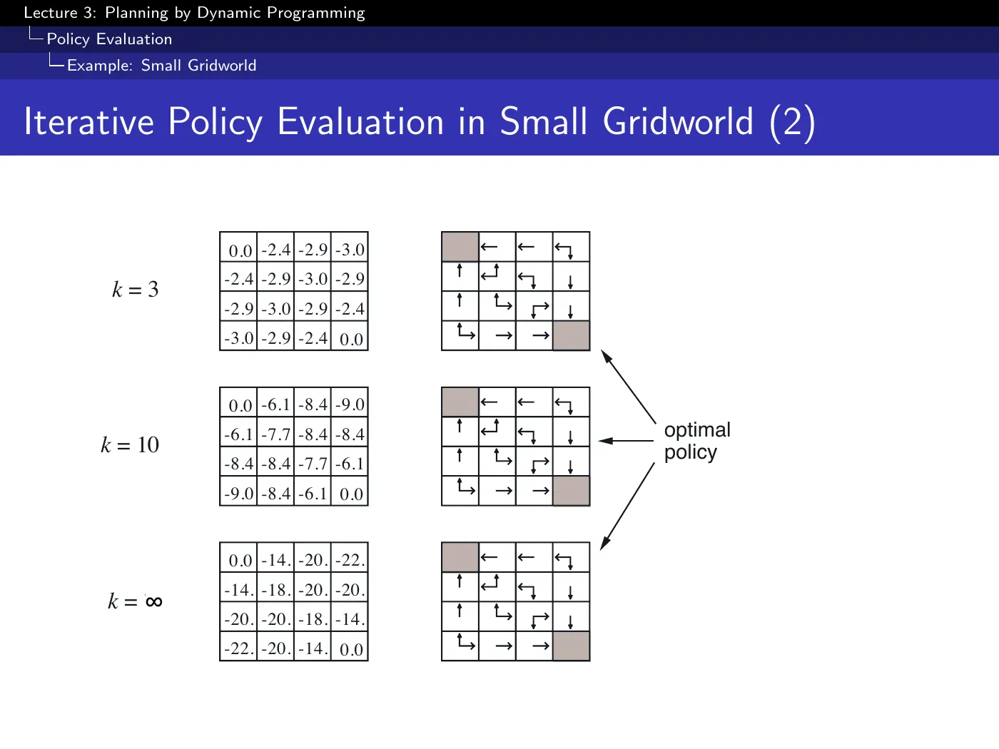
The left column is policy evaluation converging to at . The right column asks a different question: if I acted greedily with respect to , what policy would I get?
By the greedy policy is already optimal — while the value function is still nowhere near converged. Iterations 4 through compute more accurate numbers that change the greedy policy not at all.
Two consequences, and the lecture builds both: (1) any value function can be used to produce a better policy — you do not need ; (2) running evaluation to convergence is usually wasted work. That is modified policy iteration (p.18) and, pushed to the limit, value iteration.
3 · Policy iteration
p.12–13 · Evaluate, Improve, Repeat ⏱ 29:41
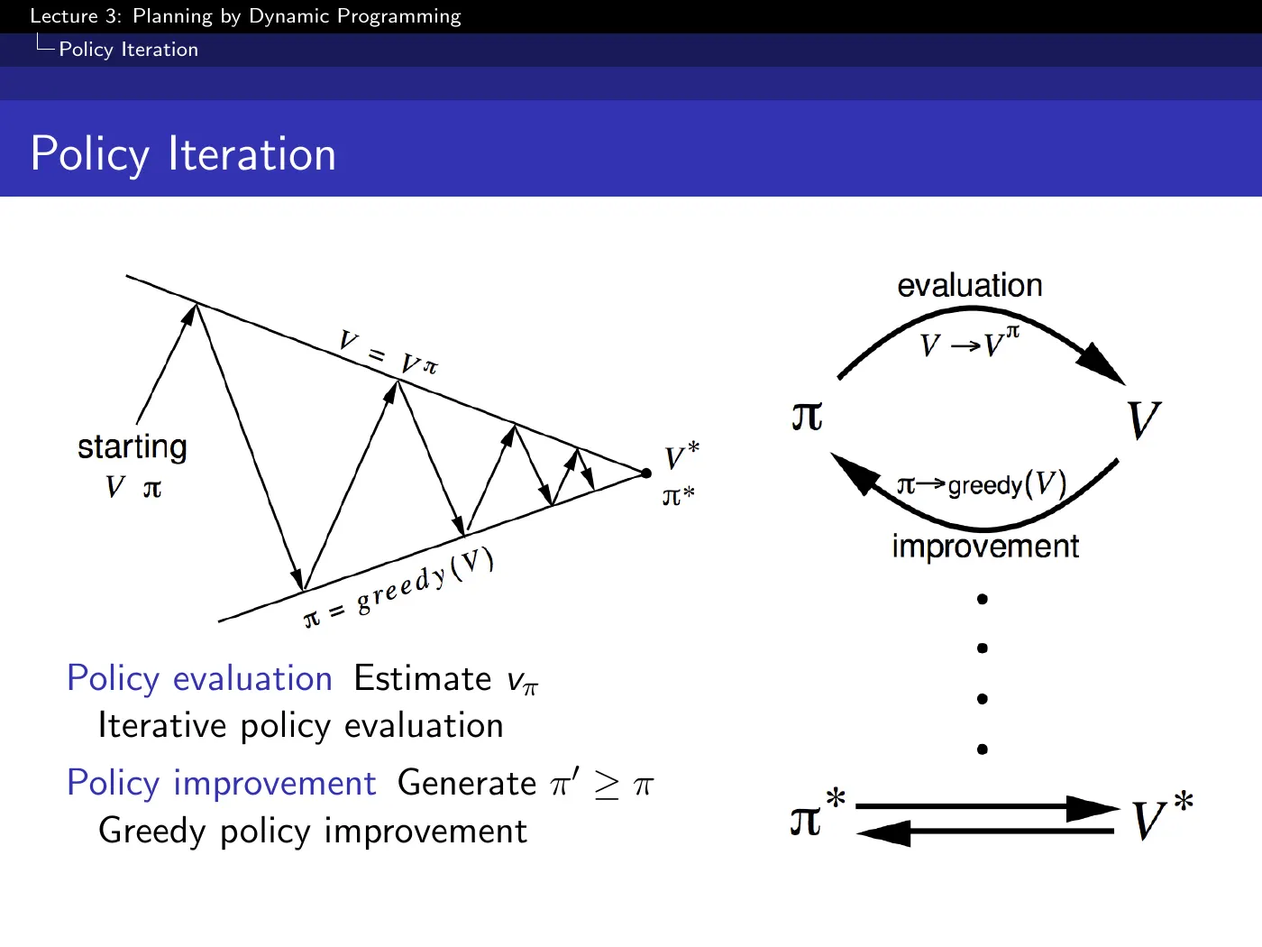
Up-arrows evaluate, down-arrows act greedily, and the two converge on and from any starting point.
Two facts the slide does not state:
- After the first improvement your policy is deterministic and stays deterministic, because returns a single action. That is consistent with the L2 theorem that a deterministic optimal policy always exists, so restricting the search to deterministic policies costs nothing.
- The convergence rate is independent of the initialization, though the initialization obviously affects how much work you do in practice — start at and you finish immediately.
This diagram is the one to memorize. It recurs in L5 with sampled evaluation, in L6 with function approximation, and in L7 with a gradient step replacing the greedy jump.
p.14–15 · Jack's Car Rental ⏱ 36:34
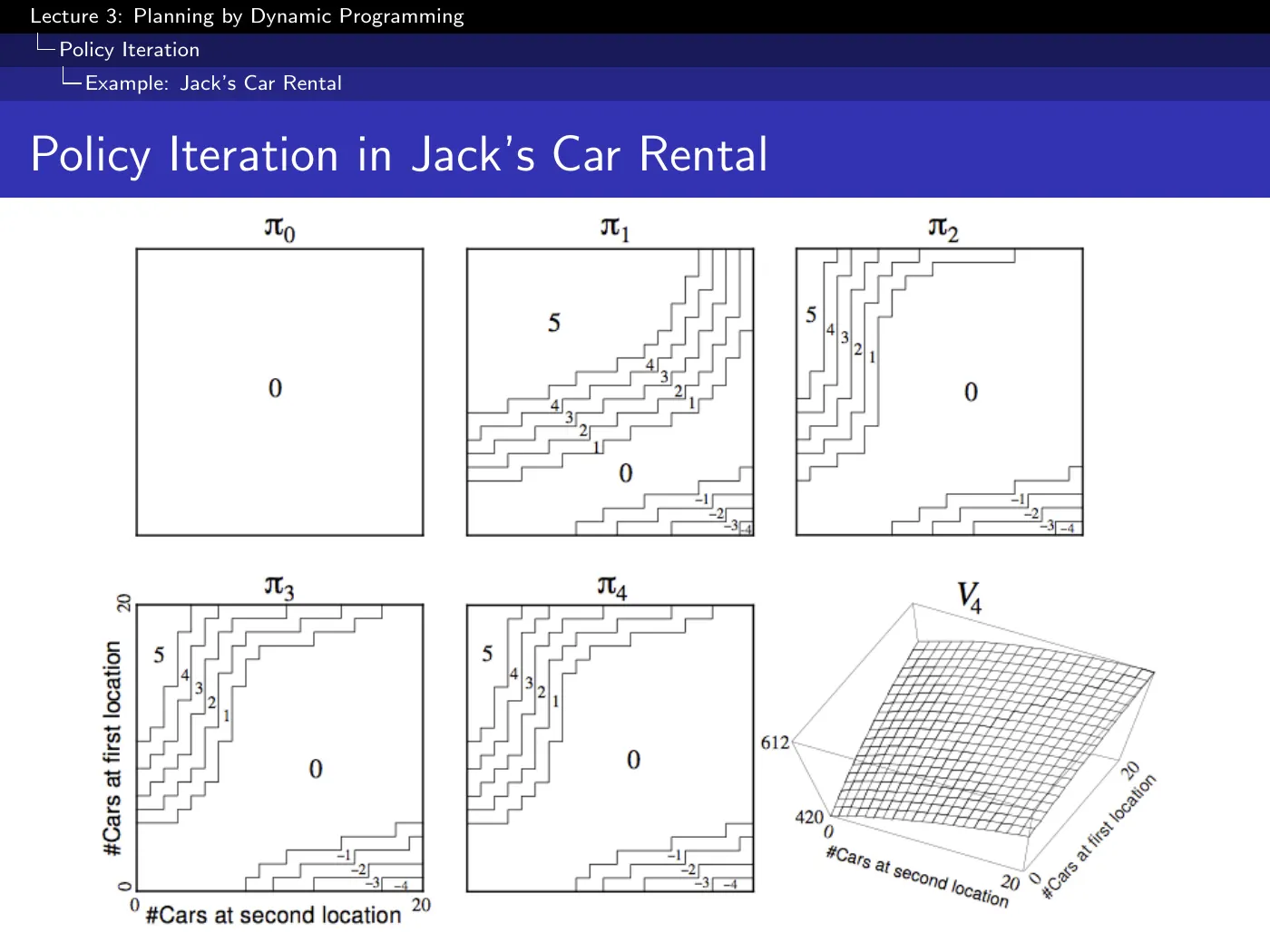
Two rental locations, up to 20 cars each, move up to 5 overnight, $10 per car rented, Poisson demand and returns. Location 2 receives more requests than returns, so it drains — the policy has to keep feeding it.
Reading the figure: the five squares are policies drawn as contour maps — axes are cars at each location, and the contour label is how many cars to move. The surface at the end is the value function, in dollars of expected lifetime revenue.
Unlike the gridworld, one improvement step is not enough: it takes four or five iterations to stabilize.
The Poisson rates for requests and returns are . Without them there is no lookahead and no algorithm. This is planning: you supply a model, and DP returns the optimal policy for the model you supplied.
That framing is how this is actually used — industry writes down an approximate model of a system and solves it. Whether the model matches reality is a separate problem, and it is the one L4 onwards attacks.
4 · Why greedy improvement works
p.16 · The Policy Improvement Theorem ⏱ 46:30
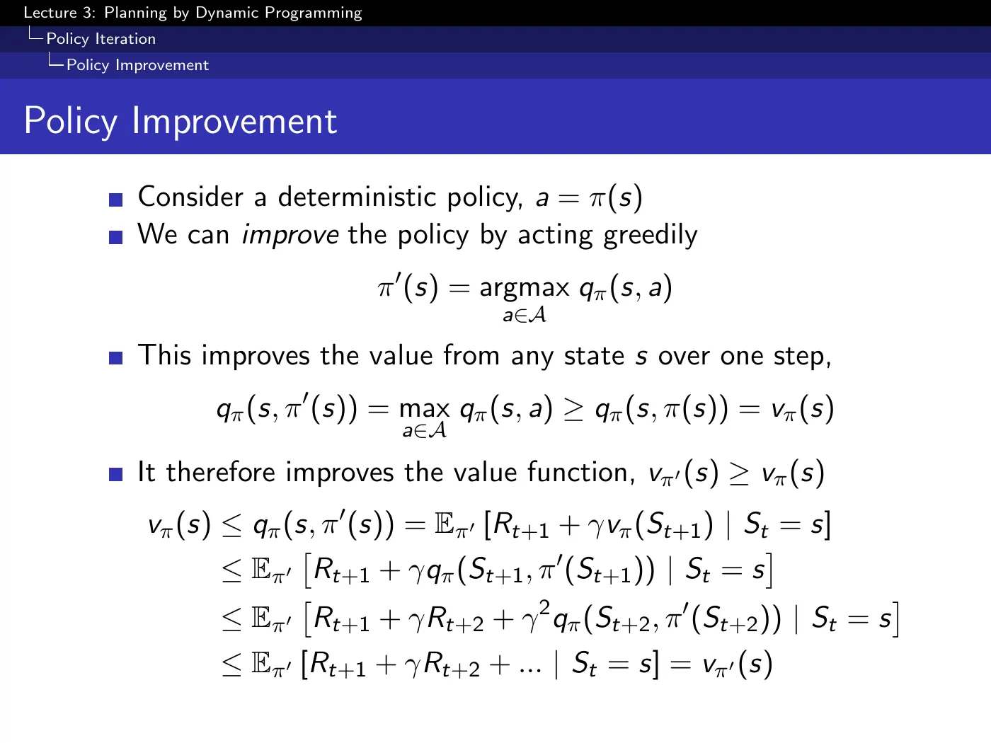
The proof is two moves, and separating them is what makes it readable.
Move 1 — one step is not worse. By construction picks the maximizing action, so
The inequality is just a max is at least as large as any particular element. What it says: follow for one step, then forever, and you do at least as well as throughout.
Move 2 — telescope it. Apply Move 1 again inside the expectation, at the next state, then again, unrolling:
Each step converts one more "then follow " into "then follow ". One step at a time is what turns a one-step improvement into a whole-policy improvement.
The commonest misreading of "act greedily" is that it optimizes immediate reward and ignores the future. It does not.
maximizes over one step of action plus the value function, and the value function already summarizes all future reward under . So greedy improvement is a one-step lookahead into a long-horizon summary — it will happily accept a worse immediate reward for a better successor state.
p.17 · When Improvement Stops ⏱ 52:36
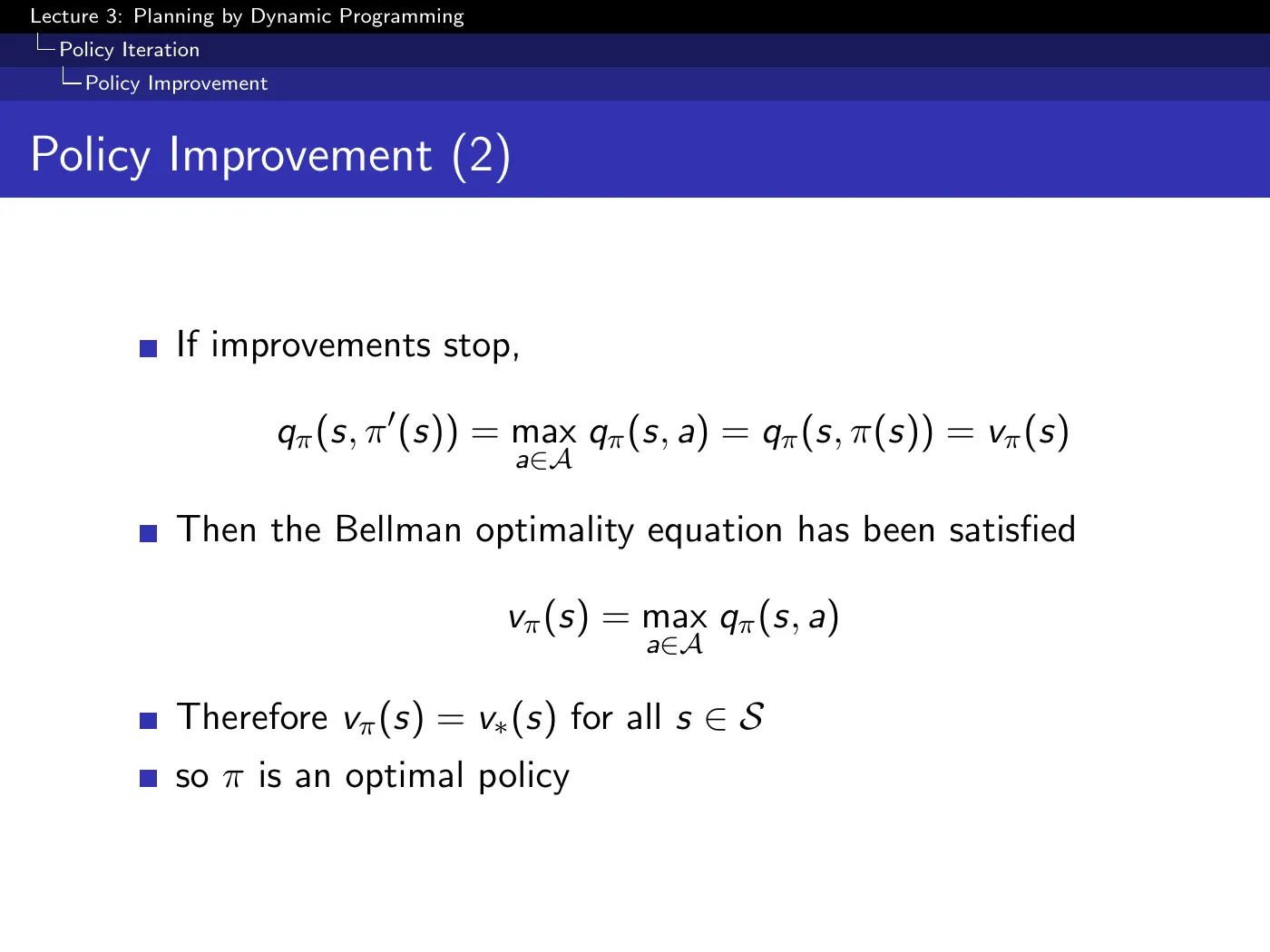
Set the inequality to equality: — which is the Bellman optimality equation. So and is optimal.
That is the whole convergence argument for policy iteration: the only way improvement can stop is by satisfying the optimality equation.
Because policy improvement defines a partial order on policies, and you can only climb it.
Write when for every state — not on average, not in most states, but everywhere. The improvement theorem guarantees each greedy step produces a policy that is its predecessor in exactly this sense.
The trap you would worry about — better in some states, worse in others — is ruled out by that "for every state". There is no sideways move to get stuck in. You climb the lattice until nothing above you exists, and by p.17 that top is .
(The finiteness of the deterministic policy set is what makes "you cannot climb forever" a termination argument.)
5 · How much evaluation is enough
p.18–19 · Modified and Generalized Policy Iteration ⏱ 58:54
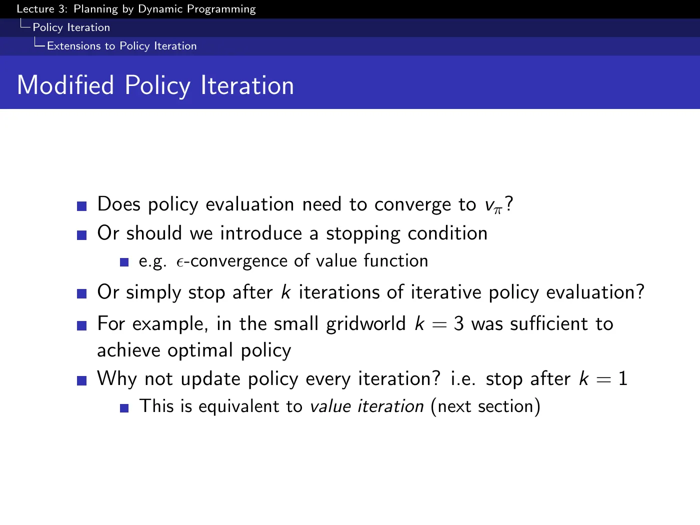
This slide answers the question the gridworld raised: must policy evaluation converge before you improve? No. Options, from most to least work: run to convergence; stop at -convergence; stop after a fixed ; stop after .
And turns out to be value iteration — evaluate once, improve, and the two collapse into a single max.
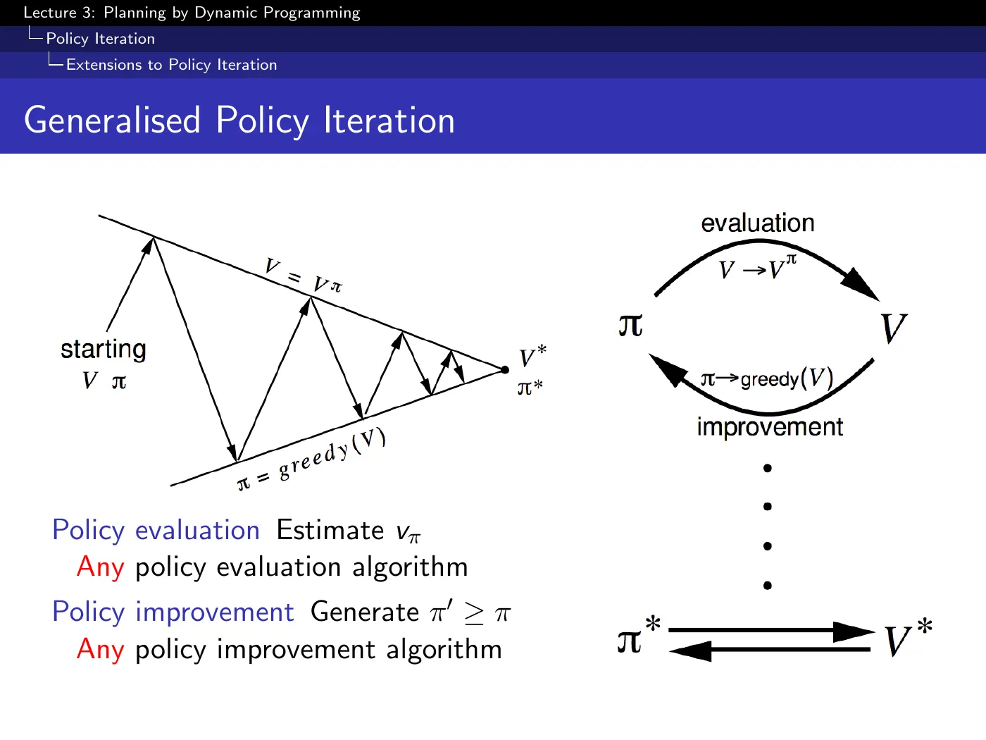
Any evaluation algorithm, any improvement algorithm, alternating. Iterative policy evaluation and greedy improvement are one instantiation among many.
Later lectures swap components in without changing the diagram: MC or TD evaluation instead of DP (L5), -greedy instead of greedy (L5), a function approximator for the value (L6), a gradient step instead of a max (L7). The picture stays; only the boxes change.
6 · Value iteration
p.20 · Principle of Optimality ⏱ 1:01:54
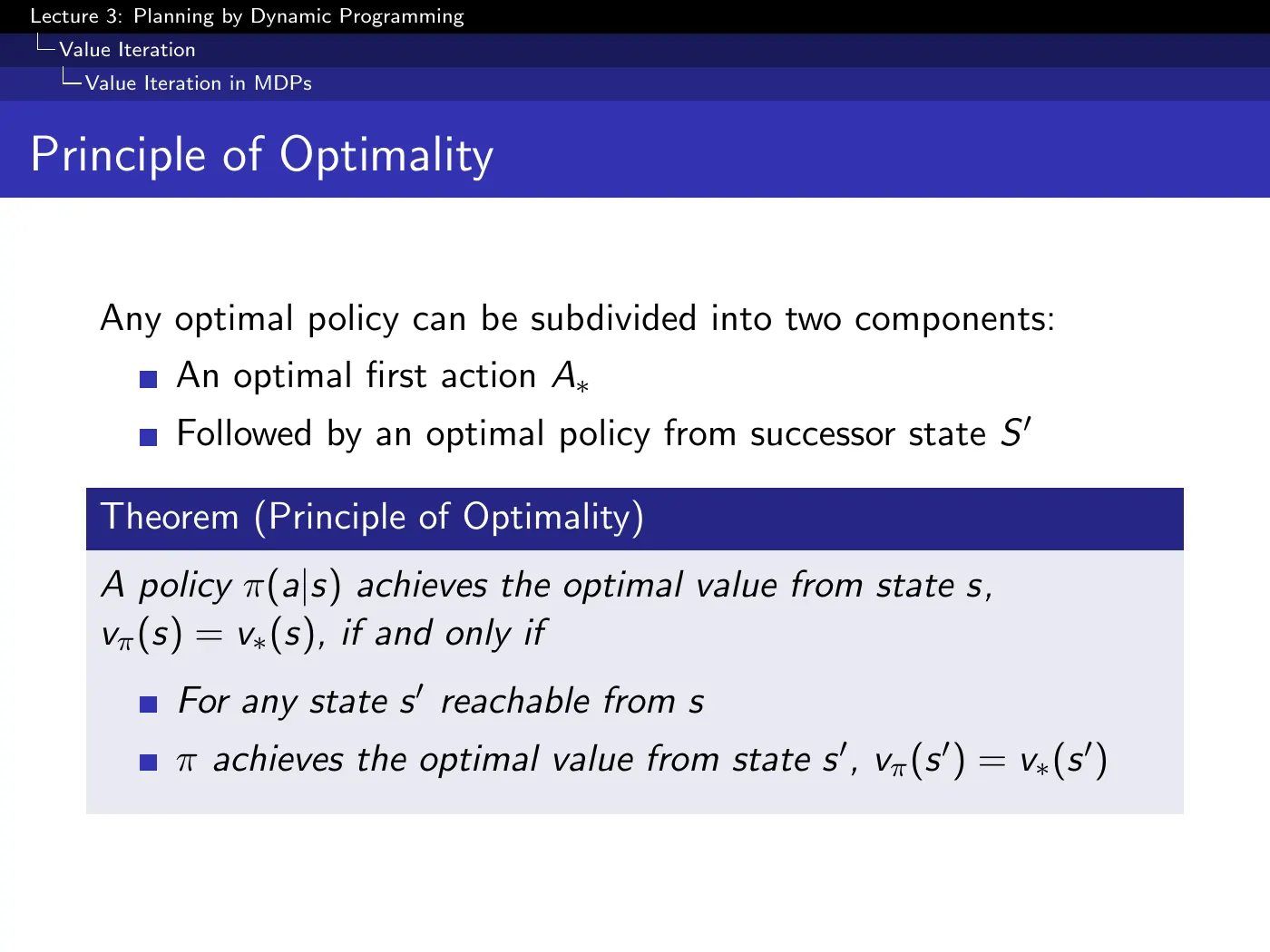
An optimal policy splits into an optimal first action and an optimal policy from wherever you land. The theorem says achieves if and only if it achieves for every reachable .
The "if and only if" is what licenses working backwards: solve the successors, then a one-step lookahead settles the predecessor.
Unreachable states are not an exception — they carry zero probability and simply do not appear in the equation.
p.21–22 · Value Iteration Intuition ⏱ 1:06:28
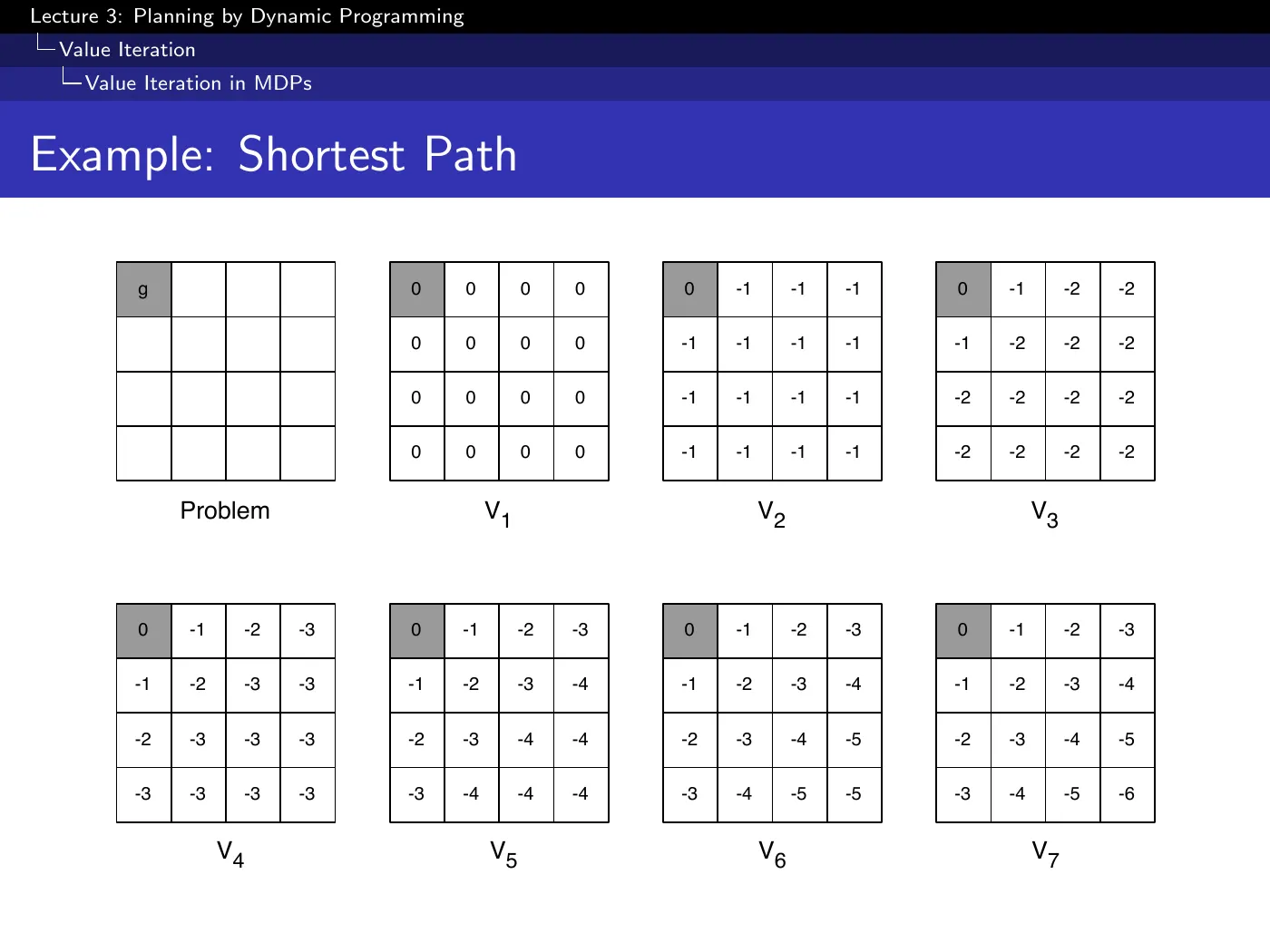
Shortest path with per step. Values propagate outward from the goal: after sweeps, every state within steps has its correct value.
The algorithm has no idea where the goal is — or whether one exists. It sweeps every state every iteration, doing the same one-step lookahead everywhere, because in general there may be no terminal state, several, or none reachable.
Value iteration works fine on continuing, looping, stochastic MDPs with discounting and no goal at all. The backwards picture is a special case that happens to be legible; do not mistake it for a requirement.
p.23–24 · Value Iteration ⏱ 1:12:38
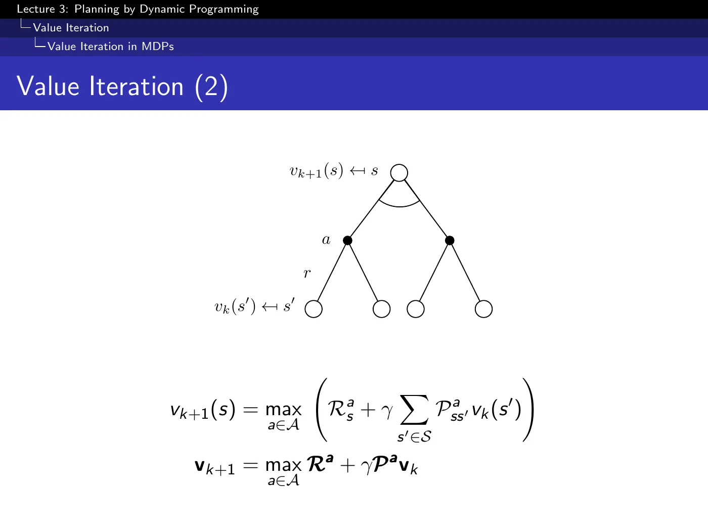
Same machinery as policy evaluation with one symbol changed: becomes . Expectation equation → optimality equation.
Policy iteration produced, at every step, the value function of an actual policy. Value iteration does not. Stop it early and is generally not for any — it is an intermediate construct, some numbers on the way to .
This resolves a genuine contradiction with p.16. The improvement theorem promised values go up; the shortest-path figure shows them going down (). Both are correct because they describe different objects: the theorem is about values of policies under policy iteration, and these are not values of policies.
Why modified policy iteration equals value iteration: evaluating the greedy () policy for exactly one step is taking the max. The two steps fuse, and no explicit policy is ever built.
7 · The summary, and complexity
p.26 · Synchronous DP Algorithms ⏱ 1:24:03
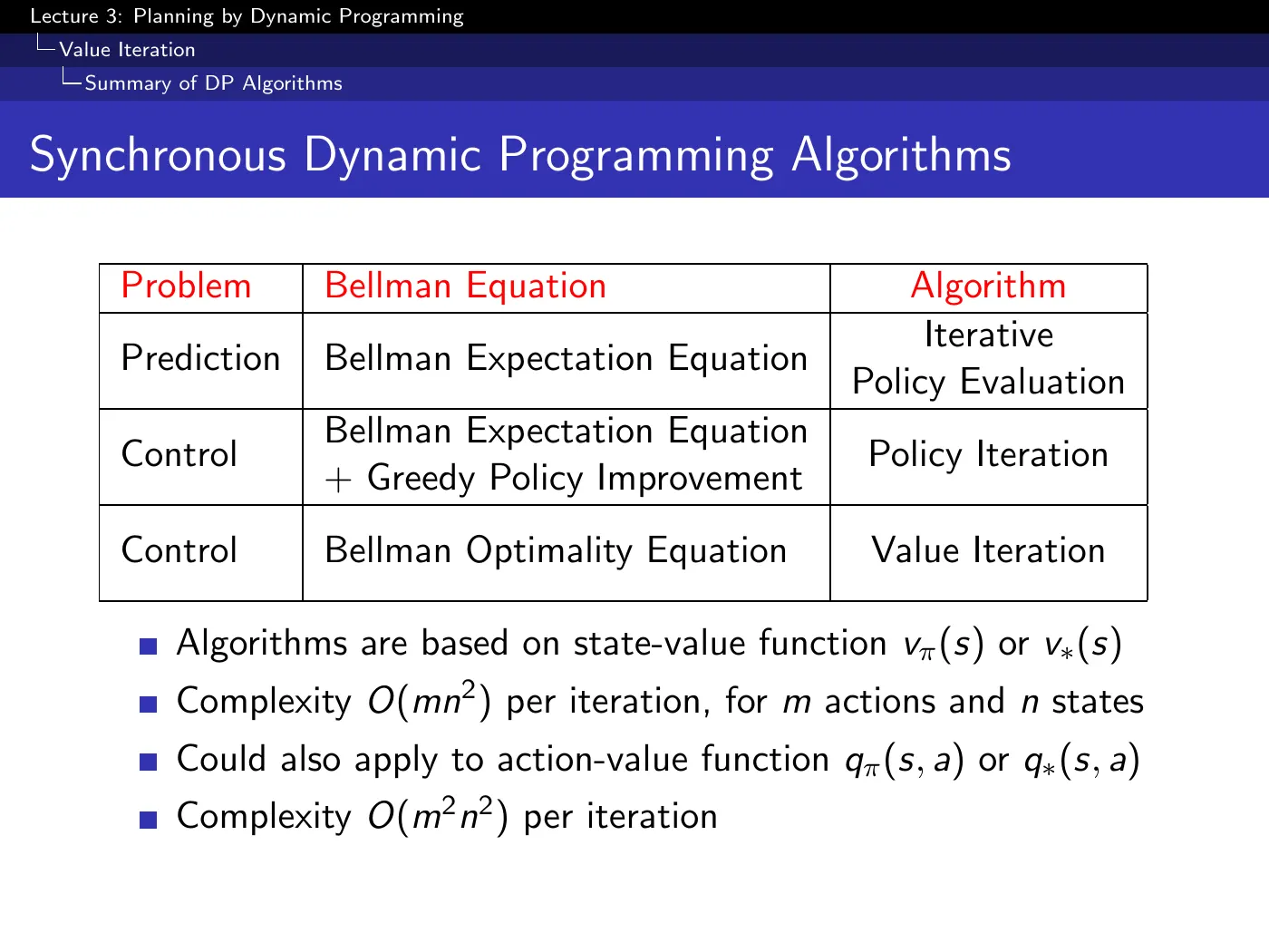
The slide the lecture asks you to take away. Three algorithms, each an iterated Bellman equation, differing only in which one.
Complexity per iteration, for actions and states:
| Using | Cost | Why |
|---|---|---|
| states as root × successors × actions | ||
| pairs as root × successor pairs |
Because removes the need for a model, and that is worth any constant factor.
Picking an action from requires a one-step lookahead — — and that lookahead is and . With it collapses to , which needs nothing but the table.
Here in L3 you were given the model, so the cheaper suffices. From L5 onward you are not, and the extra cost buys the only thing that matters → Lecture 5 · Model-Free Control. Silver flags this explicitly as coming later.
8 · Asynchronous dynamic programming
p.27–31 · Three Ways to Choose States ⏱ 1:29:27
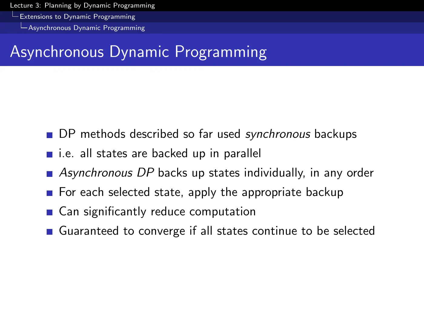
Drop the requirement that an iteration touches every state. Back up states individually, in any order.
The convergence condition is weak and worth remembering: it still converges as long as every state continues to be selected eventually. The order is free; only the coverage matters.
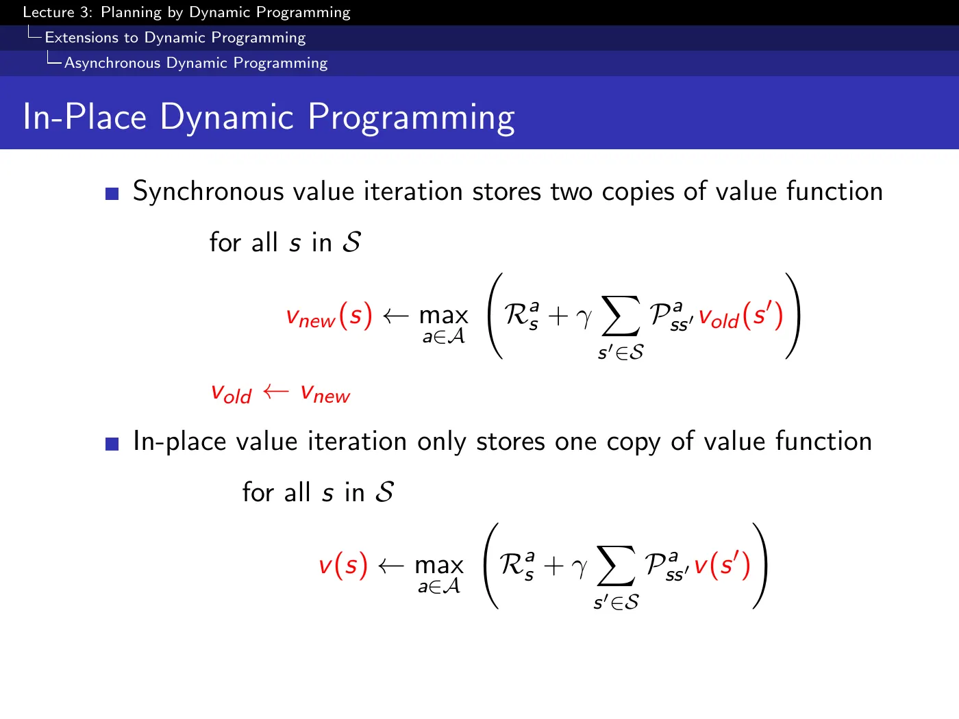
In-place keeps one copy of instead of two, so a backup immediately sees values updated earlier in the same sweep.
On a corridor, sweep from the goal backwards and in-place value iteration solves the whole thing in one sweep — each state uses the freshly-computed value of its neighbor. Sweep the other direction and you gain nothing, needing sweeps.
Same algorithm, same states, same arithmetic — only the order differs. That is the entire motivation for the next two ideas.
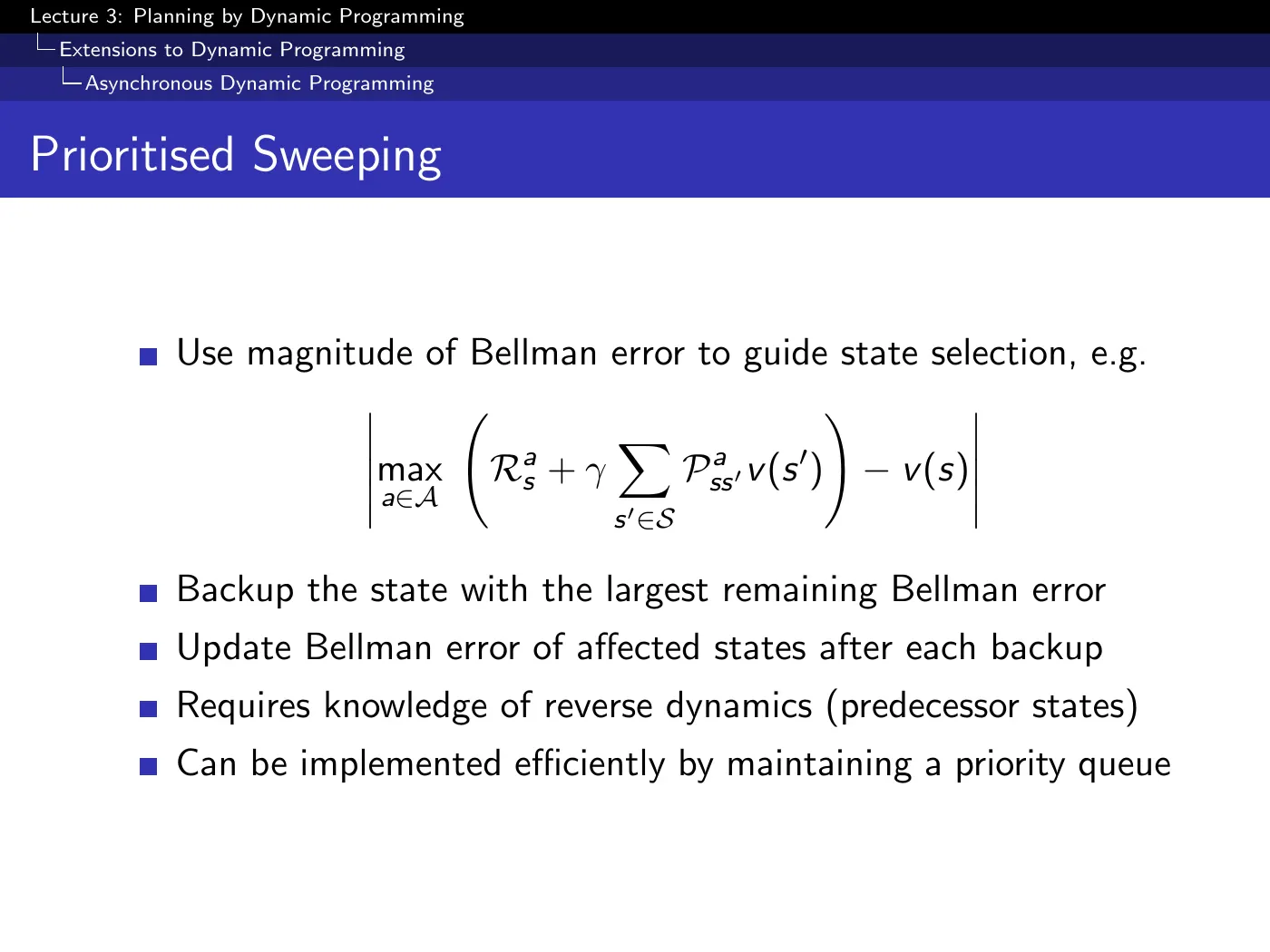
Prioritized sweeping orders by Bellman error — how much this state's value would change if updated. Large error = large downstream consequences, so do it first.
The practical picture: with rewards concentrated somewhere far away, most of the state space sits at and updating it recomputes forever. Prioritization spends effort only where something is actually changing. The cost is needing reverse dynamics — which states lead into the one you just updated — and a priority queue.
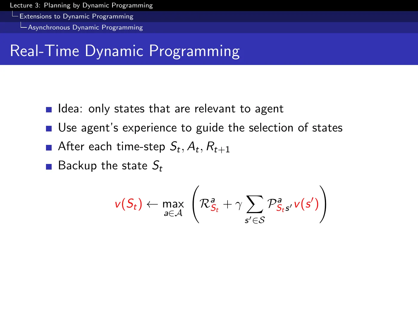
Real-time DP picks states by running the agent and backing up whatever it visits. If your robot is on this bit of carpet, the far corner of the room is not worth computing.
Using the agent's actual trajectory to decide where to compute is the seed of simulation-based search and Dyna in L8 — plan around where you are, not uniformly over everything.
Note what it is not: this is still planning. You use experience to choose where to look, but the backup itself remains a full-width expectation requiring the model.
9 · The bridge to model-free RL
p.32–33 · Full-Width and Sample Backups ⏱ 1:36:18
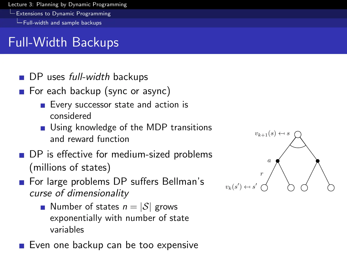
Every backup so far considered every action and every successor state. Two costs follow, and the second is the one that ends the lecture:
- Bellman's curse of dimensionality. grows exponentially in the number of state variables, so DP tops out around millions of states — fine for medium problems, hopeless for Go's , where even a single backup is unaffordable.
- You must know and . The expectation is not computable otherwise.
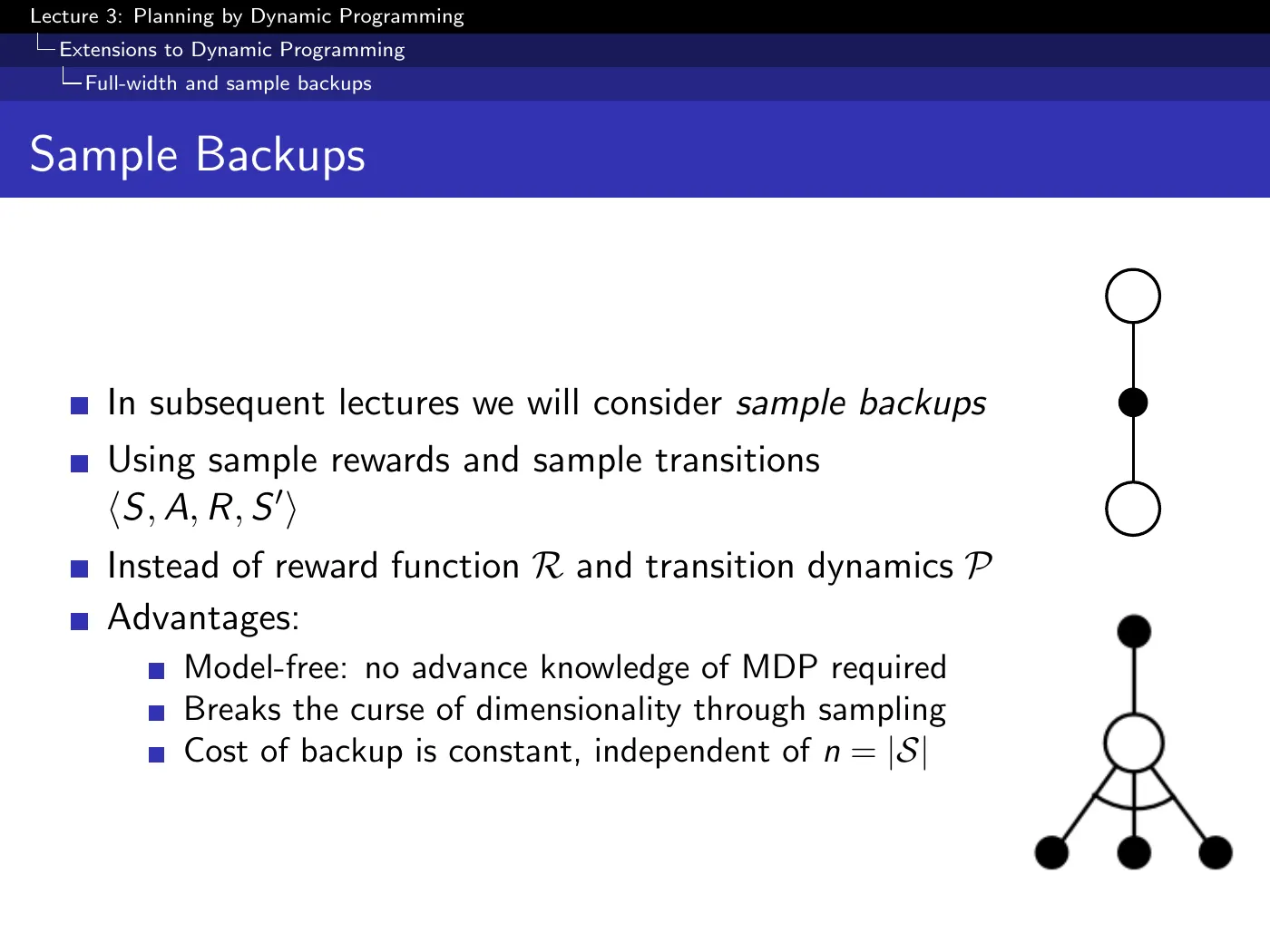
Replace the full-width expectation with a sample: take from actual interaction and back up that one transition.
- Cost becomes constant, independent of — the curse of dimensionality is broken by sampling.
- The model disappears, because you no longer compute an expectation over — you sample from the environment, which does it for you.
The second consequence is the larger one and it is almost a side effect: sampling was introduced for efficiency and delivered model-freedom. That is the transition from planning to reinforcement learning, and L4 begins on the other side of it.
Study checklist
Answer these without the notes before moving on to L4. Each item links back to where it is worked out; open the toggle only after you have tried.
1. What single operation turns L2's Bellman equations into L3's algorithms, and what does each choice give you?
→ p.7–8 · The Update ⏱ 12:56
Answer
Turn the equality into an assignment and iterate.
Bellman expectation equation → iterative policy evaluation (prediction). Expectation + greedy improvement → policy iteration. Bellman optimality equation → value iteration. That is slide p.26 and it is the whole lecture.
2. Which two properties must a problem have for DP, and what supplies each in an MDP?
→ p.3–6 · Requirements and Scope ⏱ 2:18
Answer
Optimal substructure — supplied by the Bellman equation, which decomposes a state's value into one step plus the successor's value.
Overlapping subproblems — supplied by the value function, which caches "reward obtainable from here" and is reused everywhere that state appears.
The reframe worth keeping: the value function is a cache.
3. In the small gridworld, what does the right-hand column show, and what does it imply?
→ p.9–11 · Small Gridworld ⏱ 19:45
Answer
The greedy policy with respect to . By it is already optimal, while the value function is far from converged ().
Two implications: any value function can produce a better policy — you do not need — and running evaluation to convergence is wasted work. That is modified policy iteration, and at , value iteration.
Also: is truncated for display.
4. Prove that greedy policy improvement does not make things worse, and say why greedy is not myopic.
→ p.16 · The Policy Improvement Theorem ⏱ 46:30
Answer
One step: — a max is at least any particular element. Follow once then forever and you do no worse.
Telescope: apply that inequality again at the next state, and again, converting one more "then " into "then " each time, until .
Not myopic because maximizes one step of action plus the value function, which already summarizes all future reward under . It will trade immediate reward for a better successor.
5. Why can policy iteration not get stuck at a local optimum?
→ p.17 · When Improvement Stops ⏱ 52:36
Answer
Policy improvement defines a partial order: iff in every state. Each greedy step produces a policy its predecessor in that sense, so you can only climb.
The failure you would fear — better in some states, worse in others — is excluded by the "every state" quantifier; there is no sideways move to be trapped in.
And when climbing stops, , which is the Bellman optimality equation, so is optimal.
6. Does policy evaluation have to converge before you improve?
→ p.18–19 · Modified and Generalized Policy Iteration ⏱ 58:54
Answer
No. Options: run to convergence, stop at -convergence, stop after fixed , or stop after — all converge to .
is exactly value iteration: evaluating the policy for one step is taking the max, so the two steps fuse and no explicit policy is built.
The general frame is GPI — any evaluation, any improvement, alternating — and the rest of the course swaps components into it without changing the diagram.
7. Value iteration's numbers go down while the improvement theorem says values go up. Resolve it.
→ p.23–24 · Value Iteration ⏱ 1:12:38
Answer
They describe different objects. The improvement theorem is about the value functions of actual policies under policy iteration, which do increase.
Value iteration's intermediate is generally not for any policy — it is an intermediate construct on the way to , so no monotonicity claim was ever made about it.
Policy iteration produces a real policy's value at every step; value iteration works directly in value space and never builds a policy until the end.
8. State the principle of optimality and say why "work backwards from the goal" is only intuition.
→ p.20 · Principle of Optimality ⏱ 1:01:54
Answer
achieves if and only if it achieves for every reachable . The "only if" is what lets you solve successors first and settle the predecessor with a one-step lookahead.
The algorithm does not know where the goal is — or whether one exists. It sweeps every state every iteration and works on continuing, looping, stochastic MDPs with no terminal state at all. The backwards picture is a legible special case, not a requirement.
9. Give the complexity of DP with and with , and say why the course later prefers the expensive one.
→ p.26 · Synchronous DP Algorithms ⏱ 1:24:03
Answer
per iteration with ; with — because 's roots and leaves are both state-action pairs.
removes the model. Acting from needs , and that lookahead is . With it is and needs nothing.
In L3 you have the model, so is cheaper and sufficient. From L5 you do not, and the constant factor is trivially worth paying.
10. Name the three asynchronous DP schemes and the condition that keeps convergence.
→ p.27–31 · Three Ways to Choose States ⏱ 1:29:27
Answer
In-place (one copy of , so backups see values updated earlier in the same sweep), prioritized sweeping (order by Bellman error; needs reverse dynamics and a priority queue), real-time DP (back up the states the agent actually visits).
Condition: convergence holds as long as every state continues to be selected eventually — the order is entirely free.
Ordering is worth a factor of : on a corridor swept goal-backwards, in-place value iteration finishes in one sweep.
11. What two problems do full-width backups have, and what single change fixes both?
→ p.32–33 · Full-Width and Sample Backups ⏱ 1:36:18
Answer
(1) Bellman's curse of dimensionality — grows exponentially in the number of state variables, and for large problems even one backup is unaffordable. (2) You must know and to compute the expectation.
The fix is sampling. Back up a sampled transition instead of expanding the full expectation: the cost becomes constant in , and the model disappears because the environment performs the expectation for you.
Sampling was introduced for efficiency and delivered model-freedom as a side effect. That is the step from planning to RL.
Gaps to close on your own
The lecture ran out of time and points you to the notes. This is the block that answers the questions raised and postponed twice during the lecture: does a solution exist, is it unique, do these iterations reach it, and how fast?
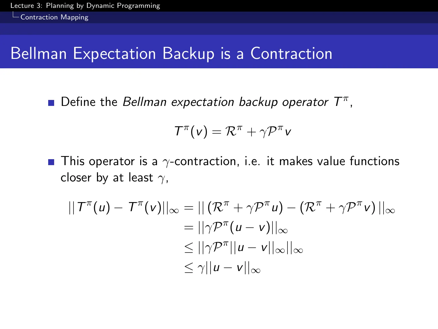
The argument in one line: measure distance between value functions by the -norm , then show the Bellman backup operator is a -contraction — it shrinks that distance by at least every application. The contraction mapping theorem then delivers a unique fixed point and a linear convergence rate of , all at once.
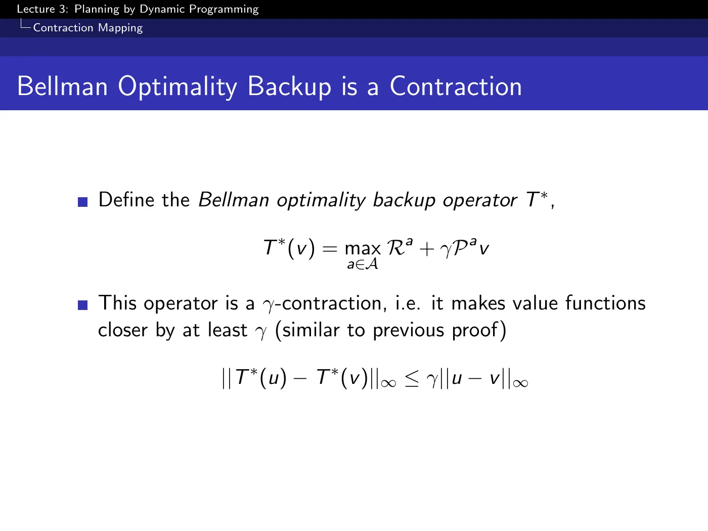
The same argument covers both operators: has fixed point (giving iterative policy evaluation and policy iteration), and has fixed point (giving value iteration).
You already had this section made permanent → Contraction Mapping & Bellman Convergence.
- Slide p.34, approximate dynamic programming, is passed over. It is the first appearance of a function approximator in the course: sample a subset of states, compute Bellman targets for them, fit the approximator, repeat — fitted value iteration. This is the direct ancestor of L6, and of DQN's fixed Q-targets in particular.
- The value iteration demo (
cs.ubc.ca/~poole/demos/mdp/vi.html) is recommended and not shown. It is the same gridworld at a size where you can watch values propagate. - Modified policy iteration's convergence for general is asserted and not proved; only the case is identified with value iteration.
- Prioritized sweeping needs reverse dynamics — the predecessors of a state. In a learned or sampled setting that is not free, and the lecture does not say how to get it.
- The relationship between policy iteration and expectation-maximization is mentioned as real but subtle, explored in recent papers, and left there.
Language notes
Phrasings worth stealing for your own technical writing and talks:
| Expression | Use |
|---|---|
| breaking them down into subproblems | the defining move of divide-and-conquer |
| a cache of everything we've figured out | reframing a data structure by what it saves you |
| each state gets a turn at being the root | describing a sweep without pseudocode |
| how much juice you can get out of it | informal gloss on a value function |
| turn the equation into an iterative update | converting a fixed-point condition into an algorithm |
| that gained us zero information | computation that ran but changed no decision |
| you can only climb | a monotone process that cannot get stuck |
| it's just an intermediate construct | a quantity with no interpretation outside the algorithm |
| the ordering really matters | same operations, different cost, by scheduling alone |
| breaks the curse of dimensionality through sampling | trading exhaustiveness for constant cost |