Bayes and Particle Filters

시리즈 첫 강의: L1 · Joint, Marginal, and Conditional · 마지막 강의: L7 · Resampling and SIR

이 문서는 시리즈의 입구입니다. 일곱 강의가 각각 어떤 질문에 답하는지, 어떤 순서로 읽는지, 기호가 무엇을 뜻하는지를 한곳에 모았습니다.

형광펜: 정의·핵심 · 직관·메커니즘 · 조건·주의

이 시리즈가 답하는 질문

이 시리즈의 목표는 Bayes filter의 두 식과 SIR particle filter의 loop를 외우지 않고 읽는 것입니다. 여기서 읽는다는 것은 각 항이 어떤 model에서 오는지, 각 등호에 어떤 법칙이 쓰였는지, 적분이 어떤 변수를 없애는지를 말할 수 있다는 뜻입니다.

\overline{\mathrm{bel}}_t(x_t) = \int p(x_t \mid x_{t-1})\,\mathrm{bel}_{t-1}(x_{t-1})\,dx_{t-1}

\mathrm{bel}_t(x_t) = \eta\,p(y_t \mid x_t)\,\overline{\mathrm{bel}}_t(x_t)

첫 식은 prediction입니다. $\mathrm{bel}_{t-1}(x_{t-1}) = p(x_{t-1} \mid y_{1:t-1})$ 에 transition model $p(x_t \mid x_{t-1})$ 을 곱하고, $dx_{t-1}$ 적분으로 이전 state를 없애면 $x_t$ 에 대한 distribution이 남습니다. 둘째 식은 update입니다. $\overline{\mathrm{bel}}_t$ 에 새 measurement $y_t$ 의 likelihood $p(y_t \mid x_t)$ 를 곱한 뒤, $\eta$ 를 곱해 전체 합(continuous state이면 적분)이 1이 되게 합니다.

두 식은 L3 §5의 두 가정(full form Markov assumption과 measurement의 conditional independence) 아래에서 성립합니다.

Particle filter는 같은 recursion을 belief 함수 대신 particle 집합으로 수행합니다. 시리즈 끝에서 읽을 수 있어야 하는 loop는 다음과 같습니다.

initialize : x_0[i] ~ p(x_0)                  for i = 1..N
for t = 1, 2, ...
    propagate : x_t[i] ~ p(x_t | x_{t-1}[i])  for i = 1..N
    weight    : w[i] = p(y_t | x_t[i])
    normalize : wbar[i] = w[i] / (w[1] + ... + w[N])
    estimate  : E[f(x_t) | y_{1:t}]
                  ≈ sum_i wbar[i] * f(x_t[i])
    resample  : a[i] ~ Categorical(wbar)      for i = 1..N
                x_t <- (x_t[a[1]], ..., x_t[a[N]])

propagate는 prediction 적분을, weight와 normalize는 likelihood 곱과 $\eta$ 를 particle 위에서 근사합니다. Exact Bayes filter에 대응하는 단계가 없는 것은 resampling뿐입니다. 그 대응은 L7 §8에서 표로 정리합니다.

모든 확률식에 던지는 세 질문

합이나 적분은 어떤 변수를 없애는가. Bar 뒤에는 무엇이 주어져 있는가. Joint를 conditional × marginal로 쪼갠 곳은 어디인가. 이 세 질문은 L1 §9에서 정리하고, 이후 모든 유도가 이 질문에 답하는 방식으로 쓰였습니다.

공부하면서 실제로 막혔던 질문

아래 질문들은 이 시리즈의 원본 공부 과정에서 나온 것입니다. 각 질문의 답이 있는 section을 붙였습니다.

Prior, likelihood, evidence는 실제로 아는 값인가. 각각 누가 주는가. → L2 §5
Prior는 어떻게 아는가. "이전에 localization을 했다"는 것은 무슨 뜻인가. → L2 §6
$x_t$ 는 $x_{t-1}$ 만 알면 되는데, 과거 measurement $y_{1:t-1}$ 는 왜 여전히 필요한가. → L3 §6
$x_0 \to x_1 \to x_2$ 아래에 $y_t$ 가 달린 그림은 제어공학의 state-space model이나 block diagram과 같은 것인가. → L3 §7
Particle은 정확히 어떤 distribution에서 어떤 방식으로 뽑는가. → L5 §5, L5 §6
$p(y)$ 는 왜 계산하기 어려운가. Unnormalized target $\tilde p$ 로 쓰면 그 계산이 쉬워지는가. → L4 §7, L6 §4
Weighted particle set에 쓰는 $\delta$ 는 Signals & Systems의 $\delta[n]$ 인가. → L6 §5
Particle의 weight는 왜 prior × likelihood가 아니라 likelihood인가. → L6 §6
$w_t^{(i)} \propto w_{t-1}^{(i)}\,p(y_t \mid x_t^{(i)})$ 는 왜 성립하는가. → L7 §1
Degeneracy는 왜 생기는가. Resampling은 계산량을 줄이는가. → L7 §2, L7 §5

강의 지도

일곱 강의는 세 묶음입니다. L1–L2는 Bayes filter에 필요한 확률 규칙만 다룹니다. L3–L4는 시간에 따라 변하는 hidden state의 model을 세우고 exact Bayes filter를 유도합니다. L5–L7은 그 filter의 적분을 sample로 근사하는 particle filter를 만듭니다.

Concept 페이지 Bayes Filter와 Particle Filter는 다른 노트가 이름으로 링크하는 짧은 페이지로, 한 줄 답, 핵심 식과 성립 조건, 강의 절 링크를 담습니다. 유도는 이 시리즈의 강의에만 있습니다.

강의	답하는 질문	핵심 식	선행
L1 · Joint, Marginal, and Conditional	Joint distribution에서 한 변수의 distribution과 conditional distribution을 어떻게 꺼내는가	$p(x)=\sum_y p(x,y)$ , $p(x,y)=p(x\mid y)\,p(y)$	고등학교 확률
L2 · Bayes Theorem	관측한 $y$ 로 $x$ 에 대한 belief를 어떻게 고치는가. 각 항은 어디서 오는가	$p(x\mid y)=\dfrac{p(y\mid x)\,p(x)}{\sum_{x'}p(y\mid x')\,p(x')}$	L1
L3 · Hidden State Models	시간이 들어간 model은 무엇으로 정의되고, 어떤 가정이 필요한가	$p(x_{0:t},y_{1:t})=p(x_0)\prod_{k=1}^{t}p(x_k\mid x_{k-1})\,p(y_k\mid x_k)$	L1, L2
L4 · The Bayes Filter	지난 belief와 새 measurement로 현재 belief를 어떻게 재귀적으로 만드는가. 왜 그대로는 계산하기 어려운가	$\mathrm{bel}_t(x_t)=\eta\,p(y_t\mid x_t)\int p(x_t\mid x_{t-1})\,\mathrm{bel}_{t-1}(x_{t-1})\,dx_{t-1}$	L2, L3
L5 · Monte Carlo and Particles	Distribution을 sample로 들고 간다는 것은 무슨 뜻인가. Particle은 어디서 오는가	$\mathbb{E}_p[f(X)]\approx\frac{1}{N}\sum_{i=1}^{N}f(x^{(i)})$ , $x^{(i)}\sim p$ i.i.d.	L4
L6 · Importance Sampling	원하는 distribution에서 직접 뽑지 못할 때 sample에 weight를 어떻게 붙이는가. Particle filter의 weight는 왜 likelihood인가	$\mathbb{E}_p[f(X)]=\mathbb{E}_q\!\left[f(X)\,\frac{p(X)}{q(X)}\right]$ (단 $p(x)>0$ 이면 $q(x)>0$ ); transition proposal을 쓰고 직전 step에서 resampling해 weight가 같을 때 $w_t^{(i)}\propto p(y_t\mid x_t^{(i)})$	L4, L5
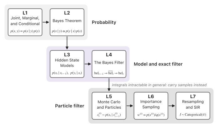
L7 · Resampling and SIR	Weight가 소수의 particle에 몰리는 이유는 무엇이고, resampling은 무엇을 고치고 무엇을 고치지 못하는가	$N_{\text{eff}}=1\big/\sum_{i=1}^{N}\big(\bar w^{(i)}\big)^2$	L6

bpf hub roadmap
화살표는 앞 강의의 결과를 뒤 강의가 직접 쓴다는 뜻입니다. 그림에는 번호가 바로 이어지는 강의 사이의 화살표만 그렸고, 한 강의를 건너뛰는 의존(예: L2 → L4, L4 → L6)은 위 표의 선행 열에 있습니다. 예를 들어 L4는 L2의 Bayes theorem과 L3의 두 가정을 함께 써서 filter를 유도합니다.

세 번 나오는 숫자 0.69

L3, L4, L5에는 같은 숫자 0.69가 일부러 반복됩니다. 과거 measurement $y_{1:t-1}$ 이 주어졌을 때 이전 state가 $A$ 일 확률이 0.3, $B$ 일 확률이 0.7이고, 각 state에서 다음 state $B$ 로 갈 transition probability가 0.2와 0.9일 때 다음 state가 $B$ 일 확률입니다.

P(x_t = B \mid y_{1:t-1}) = 0.2 \times 0.3 + 0.9 \times 0.7 = 0.69

이 등호에는 law of total probability와 full form Markov assumption $P(x_t \mid x_{t-1}, y_{1:t-1}) = P(x_t \mid x_{t-1})$ 이 쓰입니다.

L3 §6에서는 과거 measurement가 $x_{t-1}$ 에 대한 belief를 거쳐 여전히 정보를 준다는 예로 나옵니다. L4 §2에서는 prediction 합으로, L5 §6에서는 $A$ 의 particle 300개와 $B$ 의 particle 700개를 propagate했을 때 $B$ 에 도착하는 개수의 expectation $60 + 630 = 690$ 으로 나옵니다. 세 곳 모두 같은 합 $\sum_{x_{t-1}} p(x_t \mid x_{t-1})\,p(x_{t-1} \mid y_{1:t-1})$ 을 계산하고 있고, 달라지는 것은 그 합을 확률로 쓰는지 particle 빈도로 근사하는지뿐입니다.

읽는 순서와 선행 지식

번호 순서대로 읽습니다. 뒤 강의는 앞 강의 내용을 다시 가르치지 않고 해당 section으로 링크합니다.

확률은 고등학교 수준만 가정합니다. L1이 random variable부터 다시 정의하므로 따로 준비할 것은 없습니다. 대신 이미 공부한 과목과 닿는 곳이 여러 군데 있고, 그 연결은 각 강의에서 짧게 짚습니다.

이미 아는 것	쓰이는 곳	연결
Signals & Systems: Riemann sum과 적분	L1 §8	$y$ 축을 작은 구간으로 나눈 합이 $\int p(x,y)\,dy$ 가 됩니다
Signals & Systems: convolution	L4 §3	$x_t = x_{t-1}+u_t+w_t$ 에서 $u_t$ 를 알고, $w_t$ 가 density $p_w$ 를 가지며 $x_{0:t-1}$ 과 $y_{1:t-1}$ 에 independent하면, prediction 적분은 $u_t$ 만큼의 shift와 $p_w$ 와의 convolution입니다
Signals & Systems: $\delta(t)$ 와 $\delta[n]$	L6 §5	Continuous state의 weighted particle set에서 $\delta$ 는 continuous-time의 Dirac delta와 같은 대상이고, discrete state에서는 indicator $\mathbf{1}\{x=x^{(i)}\}$ 를 씁니다
제어: state-space model	L3 §7	$x_{t+1}=Ax_t+Bu_t+w_t$ 에 noise 조건을 붙이면 transition model이 됩니다. State-Space Realizations & Canonical Forms
RL: Markov property	L3 §5	Markov Decision Process (MDP)의 Markov property와 같은 생각입니다
RL: importance sampling ratio	L6 §1	Importance Sampling in Off-Policy RL의 비율과 같은 $p/q$ 형태입니다. 거기서는 trajectory 확률의 비였고, environment transition이 약분되어 각 step에서 state가 주어졌을 때의 action probability 비의 곱이 됩니다
Estimator의 bias와 variance	L5 §4	i.i.d. sample의 Monte Carlo estimator는 $\mathbb{E}_p\lvert f(X)\rvert<\infty$ 이면 unbiased이고, $\mathrm{Var}_p(f(X))<\infty$ 이면 variance가 $\mathrm{Var}_p(f(X))/N$ 입니다. Bias and Variance

RL의 Markov property와 연결할 때 한 가지를 구분해야 합니다. Bayes filter 유도에 필요한 Markov assumption은 과거 state뿐 아니라 과거 measurement까지 conditioning set에 넣은 형태 $p(x_t \mid x_{0:t-1}, y_{1:t-1}) = p(x_t \mid x_{t-1})$ 입니다. State만 넣은 형태 $p(x_t \mid x_{0:t-1}) = p(x_t \mid x_{t-1})$ 만으로는 L4 prediction 유도에 쓰는 등호 $p(x_t \mid x_{t-1}, y_{1:t-1}) = p(x_t \mid x_{t-1})$ 가 따라 나오지 않습니다. 이 차이와 반례는 L3 §5에서 다룹니다.

선형대수는 L3 §7의 행렬 notation 정도로만 쓰입니다.

기호표

기호는 시리즈 전체에서 같은 뜻으로 씁니다. 각 기호를 읽는 법은 오른쪽 열의 section에서 처음 설명합니다.

기호	뜻	설명하는 곳
$X,\ Y$ / $x,\ y$	random variable / 그 random variable이 갖는 값	L1 §2
$p(x)$	discrete이면 PMF $P(X=x)$ , continuous이면 PDF. 논문은 둘 다 $p(x)$ 로 쓰고, 이 시리즈는 차이가 중요한 곳에서 어느 쪽인지 밝힙니다	L1 §2, §7
$p(x,y)$ , $p(x\mid y)$	joint distribution, $y$ 가 주어졌을 때 $x$ 의 conditional distribution	L1 §3, §5
$x_t$ , $y_t$	시간 $t$ 의 hidden state, 시간 $t$ 의 measurement. State는 $t=0$ 부터, measurement는 $t=1$ 부터 있습니다	L3 §1
$x_{0:t}$ , $y_{1:t}$	sequence $(x_0,\dots,x_t)$ , $(y_1,\dots,y_t)$	L3 §2
$p(x_t\mid x_{t-1})$	transition model	L3 §3
$p(y_t\mid x_t)$	measurement model	L3 §3
$\mathrm{bel}_t(x_t)=p(x_t\mid y_{1:t})$	filtering belief (posterior)	L4 §1
$\overline{\mathrm{bel}}_t(x_t)=p(x_t\mid y_{1:t-1})$	predicted belief	L4 §1
$\eta$	normalization constant, $\eta^{-1}=p(y_t\mid y_{1:t-1})$	L4 §5
$\mathbb{E}_p[f(X)]$	$X$ 가 $p$ 를 따를 때 $f(X)$ 의 expectation	L5 §3
$x^{(i)}$ , $x_t^{(i)}$ , $N$	$i$ 번째 sample, 시간 $t$ 의 $i$ 번째 particle, particle 수	L5 §2
$p(x)$ , $q(x)$	importance sampling의 target, proposal	L6 §1
$\tilde p(x)$ , $Z$	unnormalized target, $Z=\int \tilde p(x)\,dx$ 이고 $p(x)=\tilde p(x)/Z$	L6 §4
$w^{(i)}$ , $\tilde w^{(i)}$ , $\bar w^{(i)}$	unnormalized weight ( $p/q$ 또는 그 상수배), unnormalized target으로 계산한 weight $\tilde w^{(i)}=\tilde p(x^{(i)})/q(x^{(i)})$ , normalized weight $\bar w^{(i)}=w^{(i)}\big/\sum_{j}w^{(j)}$	L6 §2, §4
$N_{\text{eff}}$	effective sample size	L7 §3

연산 기호도 같은 규칙을 따릅니다.

기호	뜻	설명하는 곳
$\propto$	관심 변수에 대해 상수인 배수만큼만 다르다는 뜻	L2 §4
$A\perp B\mid C$	$C$ 가 주어졌을 때 $A$ 와 $B$ 가 conditionally independent	L3 §4
$\mathcal{N}(x;\,\mu,\sigma^2)$	mean $\mu$ , variance $\sigma^2$ 인 Gaussian density를 $x$ 에서 계산한 값	L3 §3
$x^{(i)}\sim p$	" $x^{(i)}$ 를 $p$ 에서 sample한다"로 읽습니다. 근사를 뜻하는 $\approx$ 가 아닙니다	L5 §2
$\delta(x-x^{(i)})$ , $\mathbf{1}\{x=x^{(i)}\}$	continuous state의 Dirac delta, discrete state의 indicator	L6 §5
$\mathrm{Categorical}(\bar w^{(1)},\dots,\bar w^{(N)})$	index $i$ 를 확률 $\bar w^{(i)}$ 로 뽑는 distribution	L7 §4

이 시리즈에서 뺀 것

목표는 Bayes filter와 particle filter를 유도하고 읽는 것입니다. 아래 주제는 그 목표에 필요하지 않거나 따로 공부할 주제라서 뺐습니다.

Measure theory. Probability가 0인 사건에 conditioning하는 것을 엄밀하게 정의할 때 필요합니다. 이 시리즈의 유도는 density와 작은 구간 논증으로 충분하고, 그 한계는 L1 §8에서 한 문장으로 밝힙니다.
Kalman filter. Transition과 measurement가 linear이고 noise와 initial belief가 Gaussian이면(L3 §7의 noise 조건 아래) Bayes filter는 closed form을 가지며, 그것이 Kalman filter입니다. 따로 제대로 공부할 주제라서 이 시리즈에는 식을 넣지 않았습니다.
논문 응용. Lee 2020의 terrain curriculum이 SIR를 어떻게 쓰는지는 Lee 2020 · Prerequisites — Lecture Notes › 5 · Curriculum: from Bayes filter to particle filter에 있습니다. 이 시리즈는 논문 없이 읽히도록 일반적인 filter만 다룹니다.
Transition model이 아닌 proposal. $y_t$ 까지 쓰는 proposal은 한 step 안에서 생기는 proposal mismatch를 줄이는 방법입니다. Weight에 likelihood 하나만 남는 것은 transition model을 proposal로 쓰고 이전 weight가 모두 같을 때(매 step resampling한 뒤)입니다. 이 시리즈는 그 경우(bootstrap filter) 하나만 유도하고, 더 나은 proposal이 필요한 상황은 L7 §5에서 짚기만 합니다.
Particle smoothing. Smoothing은 $t$ 이후의 measurement까지 써서 $x_t$ 를 추정하는 문제입니다. 이 시리즈는 $y_{1:t}$ 만 쓰는 causal estimate인 filtering을 다루고, smoothing은 L3 §8에서 정의만 합니다.
MCMC move. Resampling 뒤 복제된 particle을 target을 보존하면서 흩뜨리는 방법인데, Markov chain Monte Carlo 이론이 따로 필요합니다. Diversity가 줄어드는 문제와 단순 jitter의 대가는 L7 §6에서 다룹니다.
Particle filter의 수렴 증명. Resampling 뒤의 particle은 independent가 아니므로 i.i.d. sample에 대한 law of large numbers로는 수렴이 바로 나오지 않고, 별도의 결과가 필요합니다. L5 §4에서 이 사실만 언급합니다.

목적성

우선순위는 🔴 practice-critical입니다. 지금 공부하는 이유는 네 가지입니다.

Lee 2020 §5가 이 filter를 씁니다. Terrain curriculum은 terrain parameter 위의 SIR particle filter(bootstrap filter)입니다. Lee 2020 · Prerequisites — Lecture Notes › 5 · Curriculum: from Bayes filter to particle filter는 prediction과 update 식, importance weight, degeneracy, sample impoverishment를 이미 아는 것으로 두고 설명합니다. 이 시리즈는 그 section을 읽는 데 필요한 수학을 처음부터 유도합니다.
Legged robot의 state estimation이 filtering 문제입니다. Base velocity처럼 policy observation에 들어가지만 직접 측정되지 않는 양은 IMU와 leg kinematics measurement로부터 추정됩니다(Sensors vs Simulator in Robot RL). 추정기가 Kalman filter 계열이든 particle filter든, prediction과 update를 번갈아 하는 구조는 L4의 Bayes filter에서 옵니다.
Probability는 논문 도중에 메우기 어려운 gap으로 이미 적혀 있습니다. Paper Reading Roadmap › What to fill with AI instead of reading a textbook은 probability를 AI가 논문 중간에 메울 수 없는 gap으로 꼽았습니다. Academic Baseline의 확률·통계 항목은 원래 "기초 ✓, 심화 약함" 한 줄뿐이었고, 이 시리즈를 공부한 2026-09-15에 개념 단위의 "첫 접촉" 항목으로 바뀌었습니다. 장기 recall은 아직 확인되지 않았습니다.
Sampling-based MPC에서도 같은 형태의 계산이 나옵니다. Paper Reading Roadmap › Sampling-based MPC, in one box의 MPPI는 sample마다 weight를 붙이고 normalize해서 weighted average를 냅니다. 이 계산은 L6의 self-normalized estimator와 형태가 같습니다. 형태가 같다는 뜻이지, MPPI weight의 의미가 particle filter의 likelihood weight와 같다는 뜻은 아닙니다.

더 읽을거리

책은 제목으로 부르고 괄호에 저자를 적었습니다. 각 자료를 어느 강의와 같이 읽으면 좋은지도 함께 적었습니다.

Probabilistic Robotics (Thrun, Burgard, Fox)는 recursive state estimation을 다루는 부분이 L1–L4에 대응합니다. 확률 기초, complete state assumption, Bayes filter 유도가 나옵니다. Nonparametric filter를 다루는 부분의 particle filter가 L5–L7에 대응하고, Gaussian filter 부분은 Kalman filter를 따로 공부할 때 읽습니다.
Bayesian Filtering and Smoothing (Särkkä)은 filtering equations를 유도하는 부분이 L3–L4에 대응합니다. Markov property를 과거 measurement까지 conditioning set에 넣은 형태로 정의합니다. Particle filtering 부분은 L5–L7에 대응하고, Monte Carlo approximation, importance sampling, SIS, SIR을 차례로 다룹니다.
A. Doucet & A. M. Johansen, "A Tutorial on Particle Filtering and Smoothing: Fifteen Years Later" (2009)는 L6–L7과 함께 읽습니다. SIS를 path space 위의 importance sampling으로 세우고 resampling을 더하는 구성이 L7 §1의 유도와 같습니다. Smoothing 부분은 이 시리즈의 범위 밖입니다.
M. S. Arulampalam et al., "A Tutorial on Particle Filters for Online Nonlinear/Non-Gaussian Bayesian Tracking", IEEE Transactions on Signal Processing 50(2), 2002(doi:10.1109/78.978374)도 L6–L7과 함께 읽습니다. SIS, degeneracy, effective sample size, resampling, 그리고 SIR filter라는 이름이 어떤 알고리즘을 가리키는지가 한 논문 안에 정리되어 있습니다.