Convex MPC for Bipedal Humanoid Locomotion

Author

Inseong Paik

Published

June 2026

Code

github.com/ispaik06/convex-mpc-biped

Stack

C++17 · MuJoCo · Eigen · OSQP · Python

Video 1The MIT Humanoid walking under the convex MPC in MuJoCo: omnidirectional velocity tracking, in-place turning, and body-pose tracking from a single controller and a single set of weights.

Abstract

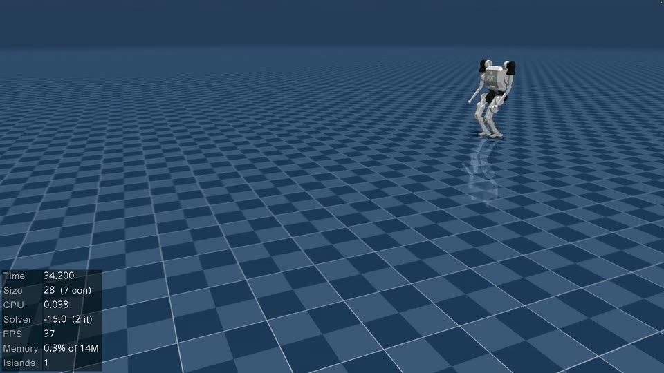
This article documents a locomotion controller I built for bipedal humanoid robots, centered on a convex model-predictive controller (MPC) over single-rigid-body (SRB) dynamics. The formulation follows the MIT Cheetah 3 controller of Di Carlo et al., but a biped is a harsher customer than a quadruped: there are only two contacts, the support region of each foot is a small rectangle rather than a point, and single-support phases leave no margin for sloppy force allocation. Moving from four point feet to two finite feet forces the decision variable from 3D contact forces to 6D contact wrenches, and forces the constraint set from a friction pyramid alone to a friction pyramid plus a center-of-pressure (CoP) support polygon and a torsional friction bound — all expressed in each foot's yaw-rotated frame.

Beyond the QP itself, most of the engineering lives in the layers around it: a receding, estimator-anchored reference trajectory that refuses to chase stale world-frame targets; a body-yaw cost transform that keeps anisotropic tracking weights physically meaningful while turning; a wrapped/unwrapped yaw policy that survives continuous rotation; Raibert-style swing-foot planning with touchdown-yaw preview and capture-point stopping; early/late contact handling that reconciles the gait schedule with measured contact; and OSQP solver engineering (structure-exploiting sparsity, contact-signature cold starts, shifted warm starts) that keeps the solve fast at 500 Hz control rates. Every MPC solve can be captured as a self-contained JSON snapshot and replayed offline through four independent verification layers. The result walks, turns in place, and tracks body pose on the MIT Humanoid in MuJoCo, and retargets to the Unitree G1 and H1 through robot-specific bindings and YAML tuning alone.

• 6D contact-wrench MPC with CoP constraints. Full derivation of the rectangular support-polygon constraint for a yaw-rotated foot, from $x_{\mathrm{cop}} = -M_y/F_z$ to the sparse world-frame constraint matrix the solver actually touches.
• Frame discipline. A deliberate split between world-frame dynamics, body-yaw command and cost semantics, and foot-frame contact geometry — including a convexity-preserving yaw-dependent cost transform and an unwrapped-yaw policy for the MPC state.
• Reactive contact management. Hysteresis-based contact estimation, early-touchdown freezing, late-contact ground search, contact-force ramping, and a near-term MPC horizon override that keeps the QP consistent with measured contact.
• Solver engineering. Row-level sparse constraint patterns, direct sparse fills without dense intermediates, contact-signature-triggered cold starts, and shifted warm starting.
• Reproducible debugging. Single-keystroke MPC snapshots replayed through four verification layers: SRB reconstruction, wrench-realizability projection, a MuJoCo contact probe, and a full receding-horizon closed-loop replay.

1Introduction

Making a humanoid robot walk is a control problem with an unusually hostile structure. Four properties conspire against you:

• Floating-base dynamics. The torso is not bolted to anything. It moves freely in $SE(3)$ and can only be stabilized indirectly, through whatever forces the feet can exert on the ground.
• Underactuation. There is no actuator on the center of mass. During single support — most of a walking cycle — the system is fundamentally underactuated, and the controller must plan through the underactuation rather than fight it.
• Hybrid contact dynamics. Every touchdown and liftoff switches the dynamics model. The controller must reason about a sequence of contact configurations, not a single smooth system.
• A small support region. A quadruped in trot still spans a support line between diagonal feet; a biped in single support balances on one foot a few centimeters wide. Feasible contact wrenches live in a thin cone, and constraint violations turn directly into foot roll and falls.

Model-predictive control is a natural answer to the first three properties: predict the body motion over a horizon that covers upcoming contact switches, and optimize contact forces subject to the physics of friction. The catch has always been speed. Nonlinear whole-body MPC is expensive and its solvers come with few guarantees; a controller that occasionally fails to return a force is not a controller you can stand on.

The MIT Cheetah 3 controller of Di Carlo et al. [1] showed how much of the problem survives aggressive simplification. Model the robot as a single rigid body driven by ground-reaction forces; linearize the orientation dynamics around yaw; treat the footstep locations as given by a heuristic planner. What remains is a convex quadratic program that solves to global optimality in well under a millisecond — fast enough to re-plan the entire force profile 25–50 times per second, robust enough to gallop a 45 kg quadruped at 3 m/s.

This project asks: how much of that story carries over to a biped, and what must be added where it does not? The answer occupies the rest of this article. The short version is that the SRB-plus-convex-QP skeleton transfers beautifully, but essentially every interface around it — the contact model, the constraint geometry, the reference generation, the cost frame, and the recovery behaviors — has to be rebuilt for two feet.

1.1 From quadruped point feet to humanoid wrenches

The Cheetah's feet are rubber balls: each contact transmits a pure force, and the friction cone is the entire constraint story. A humanoid foot is a rigid plate. It transmits a force and a moment — a full 6D wrench — and that moment is bounded by the geometry of the foot itself: push the center of pressure past the toe and the foot tips regardless of what the QP believed. The table below summarizes what changed relative to the reference formulation.

Table 1What transfers from the Cheetah 3 formulation and what this project replaces.

Aspect	Cheetah 3 (Di Carlo et al.)	This project
Platform	Quadruped, 12 DoF	Biped humanoids (MIT Humanoid, Unitree G1/H1)
Contact model	Point foot, 3D force $\mathbf{f}_i \in \mathbb{R}^3$	Finite foot, 6D wrench $[\mathbf{F}_i;\,\mathbf{M}_i] \in \mathbb{R}^6$
Input dimension / step	$3n$, up to 4 contacts	$12$ (two feet, forces + moments)
Force constraints	Friction pyramid, $F_z$ bounds	Friction pyramid, $F_z$ bounds, rectangular CoP polygon, torsional friction, all in the yaw-rotated foot frame
Swing-leg DoF handling	3-DoF legs, full task-space control	5-DoF legs (MIT) require a no-roll-moment equality row and wrench-realizability analysis; 6-DoF legs (G1) use the full wrench
Cost frame	World-axis diagonal weights	Body-yaw-rotated tracking cost, fixed from the reference yaw to preserve convexity
Reference	Operator velocities integrated forward	Estimator-anchored receding reference with gait-gated yaw integration
QP solver	qpOASES, dense	OSQP via OsqpEigen, structure-exploiting sparsity, signature-aware warm starts

1.2 Scope and honest framing

Everything here runs in MuJoCo with ground-truth (“cheater”) state estimation; hardware transfer, sensor-based estimation, and rough terrain are explicitly out of scope (§14). The MIT Humanoid is the primary, validated platform — its MJCF is not redistributed in the public repository — and the Unitree G1/H1 configurations are integration starting points rather than tuned results. The project was built over roughly three months as a from-scratch implementation: the simulator harness, controller stack, solver integration, debugging tools, and the web telemetry dashboard are all part of the codebase this article walks through.

How to read this article

Sections 2–3 set up the architecture and the model. Sections 4–5 are the mathematical core: the condensed QP and the contact-wrench constraint set. Sections 6–9 cover the planning and execution layers around the QP. Sections 10–12 are the systems half: solver engineering, robot-independent structure, and the debugging methodology. Results and limitations close it out. Readers who want the biped-specific mathematics can go straight to §5.

2System Architecture

The controller is organized as a strict hierarchy — planning decides, prediction optimizes, execution obeys — with one non-negotiable invariant: every layer consumes the same contact schedule and the same motion reference. Most walking-controller bugs I encountered were not bugs inside a layer but disagreements between layers about who is in contact and where the body is supposed to be; the architecture exists to make such disagreements structurally hard to write.

Figure 1The three-layer control hierarchy. The ContactManager sits between planning and prediction as a reactive overlay: it can override both the swing-foot targets and the near-term MPC contact schedule when measured contact disagrees with the nominal gait (§7).

2.1 Runtime loop

One process runs everything. SimulationRunner owns the MuJoCo model and steps physics at 500 Hz; on every step it refreshes the cheater-state estimate, runs RobotRunner — which drives leg/arm initialization and then the controller proper — and applies the composed torque command back to the actuators. Inside MyController::runController() the per-tick sequence is fixed:

1. synchronize the LocomotionFSM and the horizon clock;
2. filter the user command and update the body pose target;
3. query the SwingFootPlanner for nominal touchdown targets;
4. let the ContactManager reconcile scheduled vs. measured contact and possibly override those targets;
5. advance the swing trajectories;
6. if this tick is a scheduled solve boundary: rebuild reference, SRB matrices, constraints, and solve the QP;
7. write leg commands — stance legs get the newest optimal wrench, swing legs get trajectory-tracking commands.

Table 2Execution rates in the current MIT Humanoid tuning. All timing is YAML-driven; the MPC solve cadence is iterations_between_solve = 7 control ticks.

Layer	Rate	Period
MuJoCo physics integration	500 Hz	2 ms
State estimation + controller tick	500 Hz	2 ms
Contact management + swing update	500 Hz	2 ms
Leg / arm torque generation	500 Hz	2 ms
MPC solve + reference rebuild	≈71.4 Hz	14 ms
MPC prediction grid ($\Delta t$, horizon $H{=}25$)	50 Hz	20 ms × 25 = 0.5 s

Design note — two clocks, deliberately decoupled

The solve cadence (every 7 ticks, 14 ms) and the prediction grid (20 ms) are intentionally different knobs. The horizon spacing is tied to the gait — 25 samples at 20 ms cover exactly one 0.5 s gait cycle — while the solve rate is tuned to how quickly the robot must react to disturbances. A HorizonClock keeps the horizon sample times anchored to a consistent cycle origin so that gait phase, constraint schedule, and reference all agree on what time step $k$ means.

3The Single-Rigid-Body Model and Frame Conventions

The predictive model deliberately forgets that the robot has legs. It sees one rigid body — the torso, carrying the full mass and a fixed body-frame inertia — acted on by gravity and by a contact wrench at each foot. For the Cheetah this approximation was justified by light legs (≈10% of total mass); a humanoid's legs are heavier, and part of this project's debugging apparatus (§12) exists precisely to measure how far reality drifts from this model before the controller stops being able to hide the difference.

3.1 State and input

The MPC state is the 13-vector

$$\mathbf{x} \;=\; \begin{bmatrix} \phi & \theta & \psi & p_x & p_y & p_z & \omega_x & \omega_y & \omega_z & v_x & v_y & v_z & g \end{bmatrix}^{\!\top}$$

— Z-Y-X Euler orientation $\boldsymbol{\Theta} = [\phi\;\theta\;\psi]^\top$ (roll, pitch, yaw), COM position $\mathbf{p}^W$, angular velocity $\boldsymbol{\omega}^W$, COM velocity $\mathbf{v}^W$, and a constant gravity state $g$ appended so that gravity enters the dynamics as part of a homogeneous linear system rather than as an affine offset. The input stacks both feet's wrenches, forces first:

$$\mathbf{u} \;=\; \begin{bmatrix} \mathbf{F}_L^W \\[2pt] \mathbf{F}_R^W \\[2pt] \mathbf{M}_L^W \\[2pt] \mathbf{M}_R^W \end{bmatrix} \in \mathbb{R}^{12}, \qquad \mathbf{w}^W = \begin{bmatrix} F_x & F_y & F_z & M_x & M_y & M_z \end{bmatrix}^{\!\top} \text{ per foot.}$$

Convention that will matter later

Each foot's moment $\mathbf{M}^W$ is expressed in world axes but taken about that foot's contact-frame origin, not about the COM. The CoP constraints of §5 and the torque mapping of §9 are only consistent because both respect this reference point; mixing it up produces wrenches that look feasible to the QP and tip the foot in simulation. The debugging contact probe (§12.3) measures its realized moment about this same point for exactly this reason.

3.2 The three-frame split

Three frames appear throughout the controller, and the discipline about which quantity lives where is one of the central design decisions of the project:

Table 3Frame assignment. World for dynamics and geometry, body-yaw for meaning, foot for contact feasibility.

Frame	Symbol	What lives here
World	$W$	SRB dynamics, COM state, touchdown positions, MPC wrench decision variables, debug markers
Body-yaw	$B$	User command semantics, nominal foot offsets, capture-point braking offsets, the meaning of planar tracking costs
Foot	$F$	Friction pyramid, rectangular CoP region, torsional friction limit

The body-yaw frame is a bookkeeping frame, not a full 6-DoF body frame: it shares the world's vertical axis and only rotates by the yaw $\psi$. Commands transform into the world frame through

$$\mathbf{v}^{W}_{\mathrm{cmd}} = R_z(\psi)\, \mathbf{v}^{B}_{\mathrm{cmd}}, \qquad R_z(\psi) = \begin{bmatrix} \cos\psi & -\sin\psi & 0\\ \sin\psi & \cos\psi & 0\\ 0 & 0 & 1 \end{bmatrix},$$

foot-frame contact quantities relate to the world through the foot yaw $\psi_F$, $\mathbf{F}^F = R_z(\psi_F)^\top \mathbf{F}^W$ (and identically for moments), and the tracking error is weighted in a frame rotated by the reference yaw (§4.3). Keeping only yaw — never roll or pitch — in these transforms avoids mixing tilt into the vertical axis of a reduced model that has no business reasoning about tilted support surfaces.

3.3 Linearized orientation kinematics

The exact relation between Euler-angle rates and world angular velocity, for Z-Y-X angles and $\cos\theta \neq 0$, is

$$\begin{bmatrix} \dot\phi \\ \dot\theta \\ \dot\psi \end{bmatrix} = \begin{bmatrix} \cos\psi/\cos\theta & \sin\psi/\cos\theta & 0\\ -\sin\psi & \cos\psi & 0\\ \cos\psi\tan\theta & \sin\psi\tan\theta & 1 \end{bmatrix} \boldsymbol{\omega}^W .$$

For walking, roll and pitch stay near zero — the reference holds them at the pose target, and the weights of Table 7 punish deviations hard — so the small-angle form is used, which is exact in yaw and first-order in tilt:

$$\dot{\boldsymbol{\Theta}} \;\approx\; R_z(\psi)^\top \boldsymbol{\omega}^W .$$

Similarly, the rotational dynamics $\tfrac{d}{dt}(\mathbf{I}\boldsymbol{\omega}) = \sum_i \mathbf{r}_i \times \mathbf{F}_i + \sum_i \mathbf{M}_i$ drop the gyroscopic term $\boldsymbol{\omega} \times (\mathbf{I}\boldsymbol{\omega})$ — small at humanoid walking speeds — and use the yaw-rotated inertia

$$\hat{\mathbf{I}}(\psi) \;=\; R_z(\psi)\, {}^{B}\!\mathbf{I}\, R_z(\psi)^{\!\top},$$

which is the world-frame inertia of the body-frame tensor ${}^{B}\mathbf{I}$ under the small-tilt assumption. Both approximations are inherited from [1]; what is not inherited is where $\psi$ comes from — each horizon step $k$ uses its own reference yaw $\psi_k$ (§4), which is what lets the same QP remain honest during sustained in-place turning at 1.3 rad/s.

3.4 Continuous-time model

Assembling the pieces, with foot lever arms $\mathbf{r}_L, \mathbf{r}_R$ (foot position minus reference body position, §6.4) and mass $m$:

$$\dot{\mathbf{x}} = A_c(\psi)\,\mathbf{x} + B_c(\mathbf{r}_L, \mathbf{r}_R, \psi)\,\mathbf{u},$$

$$A_c = \begin{bmatrix} \mathbf{0}_3 & \mathbf{0}_3 & R_z(\psi)^\top & \mathbf{0}_3 & \mathbf{0}\\ \mathbf{0}_3 & \mathbf{0}_3 & \mathbf{0}_3 & \mathbf{1}_3 & \mathbf{0}\\ \mathbf{0}_3 & \mathbf{0}_3 & \mathbf{0}_3 & \mathbf{0}_3 & \mathbf{0}\\ \mathbf{0}_3 & \mathbf{0}_3 & \mathbf{0}_3 & \mathbf{0}_3 & \mathbf{e}_z\\ \mathbf{0} & \mathbf{0} & \mathbf{0} & \mathbf{0} & 0 \end{bmatrix} \in \mathbb{R}^{13\times13},$$

$$B_c = \begin{bmatrix} \mathbf{0}_3 & \mathbf{0}_3 & \mathbf{0}_3 & \mathbf{0}_3\\ \mathbf{0}_3 & \mathbf{0}_3 & \mathbf{0}_3 & \mathbf{0}_3\\ \hat{\mathbf{I}}^{-1}[\mathbf{r}_L]_\times & \hat{\mathbf{I}}^{-1}[\mathbf{r}_R]_\times & \hat{\mathbf{I}}^{-1} & \hat{\mathbf{I}}^{-1}\\ \mathbf{1}_3/m & \mathbf{1}_3/m & \mathbf{0}_3 & \mathbf{0}_3\\ \mathbf{0} & \mathbf{0} & \mathbf{0} & \mathbf{0} \end{bmatrix} \in \mathbb{R}^{13\times12},$$

where $[\mathbf{r}]_\times$ is the skew-symmetric cross-product matrix and $\mathbf{e}_z$ routes the gravity state into $\dot{v}_z$. The two right-hand block columns of $B_c$ are the humanoid extension in its most compact form: foot moments act on the body directly through $\hat{\mathbf{I}}^{-1}$, independent of the lever arms. This is what gives a biped in single support its authority over roll and pitch — and it is exactly the channel that the CoP constraints of §5 must keep physically honest, because the model itself would happily request a moment the foot cannot deliver.

Given yaw and lever arms along the reference trajectory, $A_c$ and $B_c$ are known functions of time step, not of the decision variables — the dynamics become linear time-varying, and the MPC stays convex.

4The Convex MPC: Discretization, Condensing, and Cost Geometry

4.1 Zero-order-hold discretization

Each horizon step $k$ carries its own continuous-time pair $(A_{c,k}, B_{c,k})$, built from the reference yaw $\psi_k$ and the reference lever arms $\mathbf{r}_{L,k}, \mathbf{r}_{R,k}$. The zero-order-hold discrete model over $\Delta t = 20$ ms is computed from a truncated matrix exponential:

$$A_{d,k} \;=\; \mathbf{1} + \Delta t\, A_{c,k} + \tfrac{1}{2}\Delta t^2 A_{c,k}^2, \qquad B_{d,k} \;=\; \Delta t\, B_{c,k} + \tfrac{1}{2}\Delta t^2 A_{c,k} B_{c,k} + \tfrac{1}{6}\Delta t^3 A_{c,k}^2 B_{c,k}.$$

$A_c$ here is nilpotent-like in structure (orientation ← angular velocity ← nothing; position ← velocity ← gravity), so the truncation error at these magnitudes is negligible while avoiding a general expm — a small example of a recurring theme: the SRB structure is simple enough that exploiting it by hand beats calling the general-purpose routine.

4.2 Condensing the horizon

Rather than keeping states as decision variables with dynamics as equality constraints, the horizon is condensed: the stacked state prediction $\mathbf{X} = [\mathbf{x}_1^\top \cdots \mathbf{x}_H^\top]^\top \in \mathbb{R}^{13H}$ is an affine function of the stacked input $\mathbf{U} = [\mathbf{u}_0^\top \cdots \mathbf{u}_{H-1}^\top]^\top \in \mathbb{R}^{12H}$,

$$\mathbf{X} \;=\; A_{\mathrm{qp}}\,\mathbf{x}_0 \;+\; B_{\mathrm{qp}}\,\mathbf{U},$$

with the lifted matrices built from per-step transition products — the LTV generalization of the constant-matrix condensing in [1]:

$$A_{\mathrm{qp}} = \begin{bmatrix} \Phi_{1,0} \\ \Phi_{2,0} \\ \vdots \\ \Phi_{H,0} \end{bmatrix}, \qquad [B_{\mathrm{qp}}]_{kj} = \begin{cases} \Phi_{k, j+1}\, B_{d,j}, & j < k\\[2pt] \mathbf{0}, & j \ge k \end{cases} \qquad \Phi_{k,j} \;=\; A_{d,k-1} A_{d,k-2} \cdots A_{d,j}.$$

The payoff is size: the decision vector shrinks to the wrenches alone ($12H = 300$ variables for $H{=}25$), swing-foot wrenches are eliminated by cheap equality rows rather than extra states, and the Hessian dimension is independent of the state dimension. The cost is that $B_{\mathrm{qp}}$ is dense — which is embraced rather than fought; §10 shows where the sparsity that does exist is spent.

The tracking objective is the weighted least-squares deviation plus a wrench-magnitude penalty,

$$J(\mathbf{U}) = \big\lVert A_{\mathrm{qp}}\mathbf{x}_0 + B_{\mathrm{qp}}\mathbf{U} - \mathbf{X}_{\mathrm{ref}} \big\rVert_{L}^{2} + \lVert \mathbf{U} \rVert_{K}^{2},$$

with $L = \mathrm{diag}(Q_1, \dots, Q_H)$ and $K = \mathrm{diag}(R, \dots, R)$ block-diagonal. Expanding and dropping constants gives the standard QP data

$$\min_{\mathbf{U}}\;\; \tfrac{1}{2}\,\mathbf{U}^{\!\top} \mathbf{H}\,\mathbf{U} + \mathbf{g}^{\!\top}\mathbf{U}, \qquad \mathbf{H} = 2\big(B_{\mathrm{qp}}^{\top} L\, B_{\mathrm{qp}} + K\big), \qquad \mathbf{g} = 2\,B_{\mathrm{qp}}^{\top} L \big(A_{\mathrm{qp}}\mathbf{x}_0 - \mathbf{X}_{\mathrm{ref}}\big),$$

subject to the contact-wrench inequalities and swing-zero equalities of §5. Only the first input $\mathbf{u}_0^\ast$ is applied; the rest of the horizon exists to make $\mathbf{u}_0^\ast$ farsighted.

4.3 The body-yaw cost transform

Here is a failure mode that does not exist on a robot that mostly walks straight. Suppose the position weights are anisotropic — say lateral tracking is punished ten times harder than longitudinal, which is typical for a narrow-footed biped. With a world-axis diagonal $Q$, the cost

$$J = (\mathbf{x} - \mathbf{x}_{\mathrm{ref}})^{\!\top} Q_{\mathrm{world}}\, (\mathbf{x} - \mathbf{x}_{\mathrm{ref}})$$

means “punish world-$y$ error hard.” The moment the robot yaws 90°, that axis is now the robot's forward direction: the controller is suddenly stiff where it should be permissive and loose where it needs authority. Foot placement rotates with the heading, the tracking objective does not, and the two drift apart — the classic symptom is a robot that walks straight beautifully and feels underdamped the moment it turns.

The fix used here transforms the tracking error into the body-yaw frame at every horizon step, using the reference yaw $\psi_{\mathrm{ref},k}$ — a known constant at QP-build time:

$$\mathbf{e}_k = T_k\,(\mathbf{x}_k - \mathbf{x}_{\mathrm{ref},k}), \qquad J = \sum_k \mathbf{e}_k^{\!\top} Q\, \mathbf{e}_k = \sum_k (\mathbf{x}_k - \mathbf{x}_{\mathrm{ref},k})^{\!\top}\, \underbrace{T_k^{\!\top} Q\, T_k}_{Q_k}\, (\mathbf{x}_k - \mathbf{x}_{\mathrm{ref},k}),$$

where $T_k$ rotates exactly three blocks and leaves the rest alone:

$$T_k = \mathrm{blkdiag}\big(\,\mathbf{1}_3,\; R_z(\psi_{\mathrm{ref},k})^\top,\; R_z(\psi_{\mathrm{ref},k})^\top,\; R_z(\psi_{\mathrm{ref},k})^\top,\; 1\,\big)$$

acting on (orientation, position, angular velocity, linear velocity, gravity). Because $T_k$ depends only on the reference — never on the decision variables — each $Q_k$ is a constant positive-semidefinite matrix and the problem remains a convex QP. The Euler block stays untransformed deliberately: roll and pitch are already body-relative tilt angles, and “rotating” raw Euler errors with a planar rotation would mix conventions. In the implementation this is a per-step reweighting inside the QP assembly (bodyYawStateCost()), costing a handful of 3×3 multiplies per step.

4.4 Wrapped vs. unwrapped yaw

A subtler prerequisite for turning: the yaw entry of the MPC state must be continuous in time, not confined to $(-\pi, \pi]$. Define the wrap operator and the unwrapped heading

$$\mathrm{wrap}(\alpha) = \operatorname{atan2}(\sin\alpha, \cos\alpha), \qquad \psi_{\mathrm{unwrapped}}(t) = \psi(0) + \int_0^t \dot\psi\,d\tau ,$$

and the policy is a two-line rule with long consequences: subtract yaws across time only in unwrapped form; take shortest-path errors only in wrapped form. The MPC initial state and the reference recurrence both use unwrapped yaw — if the state estimator hands the QP $\psi_0 = +179°$ and the reference integrates to $+181°$, the error must be $2°$, not $-358°$. Feed a wrapped state into an unwrapped reference at the $\pm180°$ seam and the QP sees a phantom full-turn error, requests a violent corrective moment, and the robot falls over — a bug family this project eliminated by construction, storing both representations in the state estimate and drawing every consumer from the correct one (wrapped for UI, logs, and feedback errors; unwrapped for the MPC state, reference, and touchdown-yaw prediction).

5Contact-Wrench Constraints for a Finite Foot

This section is the heart of the biped extension. A point foot needs one physical law — Coulomb friction. A finite foot needs three: the force must stay inside the friction cone, the center of pressure must stay inside the foot, and the free yaw moment must stay inside the torsional friction budget. All three are naturally expressed in the foot frame $F$, while the QP's decision variables live in the world frame — and the resulting frame transformation is where a naive implementation quietly goes wrong.

Per horizon step, the stacked wrench variable is ordered forces-first:

$$\mathbf{u}_k = [\,\underbrace{F_{Lx}\; F_{Ly}\; F_{Lz}}_{0..2}\; \underbrace{F_{Rx}\; F_{Ry}\; F_{Rz}}_{3..5}\; \underbrace{M_{Lx}\; M_{Ly}\; M_{Lz}}_{6..8}\; \underbrace{M_{Rx}\; M_{Ry}\; M_{Rz}}_{9..11}\,]^{\!\top}_{W},$$

so each foot's 6D wrench occupies the column sets $\{0,1,2,6,7,8\}$ (left) and $\{3,4,5,9,10,11\}$ (right) — bookkeeping that matters once the constraint matrix goes sparse (§10).

5.1 Friction pyramid and normal-force bounds

In the foot frame, Coulomb friction bounds the tangential force inside a circular cone,

$$\sqrt{F_{x,F}^2 + F_{y,F}^2} \;\le\; \mu\, F_{z,F}, \qquad F_{z,F} \ge 0,$$

which is second-order and therefore linearized to the inscribed pyramid — four rows:

$$\pm F_{x,F} - \mu F_{z,F} \le 0, \qquad \pm F_{y,F} - \mu F_{z,F} \le 0.$$

Two more rows box the normal force,

$$F_{\min} \le F_{z,F} \le F_{\max},$$

with $F_{\min} = 5$ N and $F_{\max} = 1500$ N in the MIT tuning. The lower bound is not cosmetic: forcing a strictly positive normal force on every scheduled stance foot keeps the foot loaded, which stabilizes the contact and keeps the CoP constraint below well-posed — $F_z > 0$ is exactly what licenses the multiplication in §5.2. During contact transitions this bound is softened by the contact ramp (§7.5).

5.2 The center-of-pressure constraint

Figure 2Top view of the rectangular support polygon in the foot frame. The MIT Humanoid's foot is long and narrow ($a = 6.5$ cm, $b = 1$ cm), so the pitch-moment budget dwarfs the roll-moment budget — a fact the constraint matrix must encode per axis, in the correct frame.

The center of pressure is the point on the sole where the contact pressure distribution resolves to a pure force. With the wrench taken about the foot origin,

$$x_{\mathrm{cop},F} = -\frac{M_{y,F}}{F_{z,F}}, \qquad y_{\mathrm{cop},F} = \frac{M_{x,F}}{F_{z,F}},$$

(a pitch-forward moment moves the pressure toward the heel; a roll moment moves it laterally — the signs follow from $\mathbf{M} = \mathbf{r}_{\mathrm{cop}} \times \mathbf{F}$). Physical validity of the contact is precisely the CoP remaining inside the sole rectangle:

$$-a \le x_{\mathrm{cop},F} \le a, \qquad -b \le y_{\mathrm{cop},F} \le b .$$

These are ratios of decision variables — nonlinear as written. But stance already guarantees $F_{z,F} > 0$ through the normal-force bound, so multiplying through by $F_{z,F}$ is a legal, exact linearization (not an approximation):

$$\pm M_{x,F} - b\,F_{z,F} \le 0, \qquad \pm M_{y,F} - a\,F_{z,F} \le 0.$$

Four linear rows. This is the entire mathematical cost of upgrading from point feet to finite feet — the difficulty is not the algebra but the frame in which it must be applied.

5.3 Torsional friction

A flat foot resists yaw torque only through distributed tangential friction, bounded approximately by

$$\lvert M_{z,F}\rvert \;\le\; \mu_t\, F_{z,F}, \qquad \mu_t = \lambda_{\mathrm{tor}}\,\mu,$$

where $\lambda_{\mathrm{tor}}$ collapses the pressure-distribution geometry into one scale (0.0657 in the MIT tuning — of the order of the foot's characteristic radius). Without these two rows the QP will happily balance an in-place turn on yaw torque the sole cannot supply, and the stance foot pivots underneath the robot.

5.4 The per-foot template

Stacking all twelve rows against the local wrench $\mathbf{w}_F = [F_{x,F}\,F_{y,F}\,F_{z,F}\,M_{x,F}\,M_{y,F}\,M_{z,F}]^\top$:

$$C_F \;=\; \begin{bmatrix} 1 & 0 & -\mu & 0 & 0 & 0\\ -1 & 0 & -\mu & 0 & 0 & 0\\ 0 & 1 & -\mu & 0 & 0 & 0\\ 0 & -1 & -\mu & 0 & 0 & 0\\ 0 & 0 & 1 & 0 & 0 & 0\\ 0 & 0 & -1 & 0 & 0 & 0\\ 0 & 0 & -b & 1 & 0 & 0\\ 0 & 0 & -b & -1 & 0 & 0\\ 0 & 0 & -a & 0 & 1 & 0\\ 0 & 0 & -a & 0 & -1 & 0\\ 0 & 0 & -\mu_t & 0 & 0 & 1\\ 0 & 0 & -\mu_t & 0 & 0 & -1 \end{bmatrix}, \qquad \mathbf{b}_F = \begin{bmatrix} 0\\0\\0\\0\\ F_{\max}\\ -F_{\min}\\ 0\\0\\0\\0\\0\\0 \end{bmatrix}, \qquad C_F\, \mathbf{w}_F \le \mathbf{b}_F .$$

5.5 Rotating the constraints, not the variables

The QP variables are world-frame wrenches, but $C_F$ speaks foot-frame. The clean resolution is to compose the template with the world→foot rotation, producing a matrix that acts directly on world-frame variables:

$$C_W \;=\; C_F \cdot \mathrm{blkdiag}\!\big(R_{WF}^{\top},\, R_{WF}^{\top}\big), \qquad R_{WF} = R_z(\psi_F),$$

with $\psi_F$ the stance foot's yaw, read from the foot frame's $x$-axis at constraint-build time. Writing $c = \cos\psi_F$, $s = \sin\psi_F$, the full explicit result:

$$C_W = \begin{bmatrix} c & s & -\mu & 0 & 0 & 0\\ -c & -s & -\mu & 0 & 0 & 0\\ -s & c & -\mu & 0 & 0 & 0\\ s & -c & -\mu & 0 & 0 & 0\\ 0 & 0 & 1 & 0 & 0 & 0\\ 0 & 0 & -1 & 0 & 0 & 0\\ 0 & 0 & -b & c & s & 0\\ 0 & 0 & -b & -c & -s & 0\\ 0 & 0 & -a & -s & c & 0\\ 0 & 0 & -a & s & -c & 0\\ 0 & 0 & -\mu_t & 0 & 0 & 1\\ 0 & 0 & -\mu_t & 0 & 0 & -1 \end{bmatrix}.$$

The trap this design avoids

Applying the CoP bounds directly to world-frame $M_x, M_y$ is correct only when the foot yaw is exactly zero. The support rectangle is glued to the foot, not to the world and not to the torso: at $\psi_F = 90°$, the world's $x$-moment is the foot's roll channel with its 1 cm budget, not the 6.5 cm pitch budget. A controller with world-axis CoP constraints walks straight flawlessly and tips its feet the moment it turns — a bug that is invisible in exactly the tests people run first. Note also the sparsity consequence, which §10 exploits: after rotation, every friction row touches $\{F_x, F_y, F_z\}$ and every CoP row touches $\{F_z, M_x, M_y\}$.

5.6 Equality constraints: swing legs and the 5-DoF ankle

A second matrix $D$ carries the equalities, $D_k \mathbf{u}_k = \mathbf{0}$, with 12 rows per step in three roles:

• Swing-leg zeroing. If side $s$ is in swing at step $k$, identity rows pin that leg's six wrench components to zero — the gait schedule expressed as constraint structure. (The inequality rows for that foot are simultaneously deactivated.)
• The no-roll-moment row. The MIT Humanoid's leg has five actuated DoF: the ankle can pitch but not roll. A stance foot therefore cannot exert an ankle-roll moment about its own long axis. When the no_roll_moment wrench model is active, the roll-row of a stance foot is replaced by
  $$\hat{\mathbf{x}}_{F}^{W} \cdot \mathbf{M}^W \;=\; 0,$$
  the foot's current world-frame $x$-axis dotted with its moment — three coefficients in the moment columns, updated from the measured foot pose before every constraint build. Without this row the QP allocates roll moments the hardware cannot produce, and the torque mapping silently projects them away (§9.3 quantifies the resulting error).
• Stance passthrough. Stance rows not used by either role contribute nothing, but their slots remain in the sparse pattern so that stance/swing flips change only values, not structure — the detail that makes warm starting practical (§10.3).

Stacked over the horizon, the complete constraint block is

$$C \in \mathbb{R}^{24H \times 12H}, \qquad D \in \mathbb{R}^{12H \times 12H}, \qquad \underline{\mathbf{c}} \le \begin{bmatrix} C \\ D \end{bmatrix} \mathbf{U} \le \overline{\mathbf{c}},$$

with the equality rows encoded as equal lower/upper bounds in OSQP's two-sided form, and the inequality lower bounds at $-\infty$. For $H = 25$: 300 variables, 600 inequality rows, 300 equality rows — solved comfortably within a 2 ms control tick.

6Reference Trajectory: Receding, Estimator-Anchored, Gait-Aware

The reference generator answers one question for the QP: where should the body be at each of the next 25 horizon samples? Its design principle sounds obvious and is routinely violated: a velocity-commanded walker must not chase a position it accumulated in the past.

6.1 Mode-dependent seeding

Each rebuild starts from a seed state $(\psi_0, \mathbf{p}_0^W, \dots)$ chosen by mode:

• Standing seeds from the pose target — position holding is the entire job, so the reference should pull the body back to where it is supposed to stand.
• Walking seeds planar position and yaw from the current state estimate, then rolls forward under the commanded velocity. Height, roll, and pitch remain target quantities: $p_{z} = z_{\mathrm{nom}} + \Delta z_{\mathrm{cmd}}$, applied exactly once rather than integrated.

The walking choice is the important one. Suppose the robot is shoved sideways half a step. A persistent world-frame reference — one that kept integrating from where the body used to be — now demands that the MPC fight its way back to a stale line in space, spending its narrow lateral wrench budget on position recovery the operator never asked for. The receding reference instead accepts the displacement as the new origin and tracks velocity from there; foot placement (§8), which is also anchored to the estimated COM, remains consistent with the body the robot actually has, not the body the integrator remembers. After this change, push-recovery behavior stopped fighting itself — the MPC and the foothold planner finally agreed about where “here” is.

6.2 Gait-gated yaw integration

Yaw advances by recurrence along the horizon, optionally gated by the gait. The gate exists because physically, a biped turns by swinging a foot to a rotated placement — during double support with both feet planted, commanding continued rotation of the reference just winds up torsional stress against the constraint set of §5.3. The double-support predicate is sampled with a half-step lookback to avoid chattering at phase boundaries:

$$t_{s,k} = \begin{cases} t_k, & k = 0,\\[2pt] t_k - \tfrac{1}{2}\Delta t, & k \ge 1, \end{cases} \qquad g_k = \begin{cases} 0, & c_L(t_{s,k}) \wedge c_R(t_{s,k}) \quad \text{(double support)}\\[2pt] 1, & \text{otherwise,} \end{cases}$$

$$\psi_k \;=\; \psi_{k-1} + g_k\, \dot\psi_{\mathrm{cmd}}\, \Delta t .$$

The integration mode is configurable (single_support / double_support / always); the current MIT tuning integrates at every step ($g_k \equiv 1$), which — combined with the stance-foot yaw-hold moment of §7.6 and the touchdown-yaw preview of §8 — produced the smoothest sustained turning. The gated machinery remains in place as a tuning lever, and the recurrence runs on unwrapped yaw per the policy of §4.4.

6.3 Planar propagation

Position rolls forward in world coordinates, but the command is interpreted in the body-yaw frame at each step's current reference heading:

$$\mathbf{p}^W_{k+1} = \mathbf{p}^W_k + R_z(\psi_k) \begin{bmatrix}\dot x_{\mathrm{cmd}}\\ \dot y_{\mathrm{cmd}}\\ 0\end{bmatrix}\Delta t, \qquad \mathbf{v}^W_k = R_z(\psi_k) \begin{bmatrix}\dot x_{\mathrm{cmd}}\\ \dot y_{\mathrm{cmd}}\\ \dot z_{\mathrm{cmd}}\end{bmatrix}.$$

So a fixed forward command traces an arc when combined with a yaw rate — the reference is a unicycle rollout, which is exactly the motion vocabulary of the keyboard/operator interface. Each horizon sample then assembles the full reference state: roll/pitch from the pose target, $\psi_k$ from the recurrence, $\boldsymbol{\omega}_{\mathrm{ref}} = [0, 0, g_k\dot\psi_{\mathrm{cmd}}]$, velocities from the rotated command, and the gravity constant. Deliberately conservative — the reference models only the reduced-body motion the MPC needs, nothing it does not.

6.4 Foot-relative lever arms

Alongside the state reference, the builder emits per-step contact lever arms measured from the reference body position to the planned foothold positions:

$$\mathbf{r}_{L,k} = \mathbf{p}^W_{L,\mathrm{des}} - \mathbf{p}^W_k, \qquad \mathbf{r}_{R,k} = \mathbf{p}^W_{R,\mathrm{des}} - \mathbf{p}^W_k .$$

These are not swing trajectories — they are the moment arms inside $B_c$'s $\hat{\mathbf{I}}^{-1}[\mathbf{r}]_\times$ blocks (§3.4). This coupling is why reference and foothold planner must agree: shift the body reference without shifting the planned footholds and every predicted moment arm is wrong, which the QP then compensates with wrenches the real robot never needed. Keeping both anchored to the same estimated state is what makes the pair self-consistent.

7Gait Scheduling and Reactive Contact Management

Two components share responsibility for contact, and the split is deliberate: GaitScheduler is a pure function of time — the periodic plan — while ContactManager is the reactive layer that reconciles that plan with measured reality. The scheduler never lies about the plan; the manager is allowed to override it for a few ticks when the ground disagrees.

7.1 Periodic phase and the nominal schedule

With cycle time $T_c$, swing time $T_{\mathrm{sw}}$, stance time $T_{\mathrm{st}}$ ($T_c = T_{\mathrm{sw}} + T_{\mathrm{st}}$, enforced at config load), each side's phase is the fractional cycle position with a half-cycle offset between legs:

$$\varphi_s(t) = \mathrm{frac}\!\left(\frac{t - t_0}{T_c} + \phi_s\right), \qquad \phi_{\mathrm{Left}} = \tfrac{1}{2},\;\; \phi_{\mathrm{Right}} = 0,$$

$$c_s(t) = \begin{cases} 1, & 0 \le \varphi_s(t) < T_{\mathrm{st}}/T_c \quad \text{(stance)}\\[2pt] 0, & \text{otherwise} \quad \text{(swing)}, \end{cases}$$

where $t_0$ is the cycle origin maintained by the HorizonClock. Standing mode short-circuits everything to $c_s \equiv 1$. The MIT gait uses $T_c = 0.5$ s, $T_{\mathrm{sw}} = 0.17$ s, $T_{\mathrm{st}} = 0.33$ s — a stance fraction of 66%, giving a double-support overlap of

$$T_{\mathrm{ds}} = 2T_{\mathrm{st}} - T_c = 0.16\ \text{s}$$

per half-cycle (32% of the cycle in double support). That is a conservative, walking-like gait: plenty of overlap for wrench handoff between feet, at the cost of top speed.

7.2 From schedule to constraint structure

At every scheduled solve, the scheduler evaluates $c_s(t_k)$ across the horizon and emits the per-step constraint data of §5: stance flags select which inequality rows are live and which equality rows zero a swing leg, the normal-force bounds are written into the bound vector, and each stance foot's yaw (read from its measured $x$-axis) parameterizes the rotated rows. Because $H\,\Delta t$ equals one full gait cycle, the QP always sees a complete stance/swing rotation ahead — the property that lets it pre-load the incoming foot before the outgoing foot lifts.

7.3 Measured contact with hysteresis

Contact is estimated from the measured normal force with two-sided hysteresis and tick-count confirmation:

$$\hat c_{t+1} = \begin{cases} 1, & F_z \ge F_{\mathrm{on}} \ \text{for } N_{\mathrm{on}} \text{ consecutive ticks}\\[2pt] 0, & F_z \le F_{\mathrm{off}} \ \text{for } N_{\mathrm{off}} \text{ consecutive ticks}\\[2pt] \hat c_t, & \text{otherwise,} \end{cases}$$

with $F_{\mathrm{on}} = 36$ N, $F_{\mathrm{off}} = 0.5$ N in the MIT tuning — the wide gap is intentional, because grazing contact at touchdown produces force chatter precisely when a wrong contact bit does the most damage.

7.4 Early contact

The foot finds ground before the schedule expects it:

$$\mathrm{early} \;=\; (c_{\mathrm{sched}} = 0)\;\wedge\;(\hat c = 1)\;\wedge\;\mathrm{releasedDuringSwing},$$

where the third conjunct — the foot must first have reached a confirmed no-contact state during this swing — prevents residual liftoff contact from being misclassified as touchdown. On detection, four things happen in order:

1. Freeze the foothold. The commanded target snaps to the actual landing point, $\mathbf{p}^W_{\mathrm{cmd}} \leftarrow \mathbf{p}^W_{\mathrm{foot}}$ — continuing to drag a grounded foot toward a planned target only scuffs and destabilizes it.
2. Switch the leg to support mode. Swing-foot tracking hands over to stance wrench control immediately.
3. Update the near-term MPC schedule. The first $N_{\mathrm{lock}}$ horizon steps are overridden to reflect the true contact state (§7.5), so the very next solve allocates force to the foot that actually exists.
4. Ramp the load. Wrench feedforward on the new contact scales in smoothly rather than stepping.

7.5 Late contact, the contact ramp, and the horizon override

The mirror failure — schedule says stance, force says nothing — triggers ground search: the touchdown anchor freezes and the commanded target descends at a bounded rate,

$$d_{\mathrm{search}}(t + \Delta t) = \min\big(d_{\max},\; d_{\mathrm{search}}(t) + v_{\mathrm{search}}\,\Delta t\big), \qquad \mathbf{p}^W_{\mathrm{search}} = \mathbf{p}^W_{\mathrm{freeze}} - d_{\mathrm{search}}\,\mathbf{e}_z,$$

until contact is re-established or a timeout flags recovery failure. Around every contact transition, a ramp factor

$$\alpha = \operatorname{clamp}\!\left(\frac{t_{\mathrm{contact}}}{T_{\mathrm{ramp}}},\, 0,\, 1\right)$$

scales both the stance wrench feedforward in the leg controller and the effective minimum normal force inside the MPC bounds, $F_{z,\min}^{\mathrm{eff}} = \alpha F_{z,\min}$ — so the QP is never forced to demand full loading from a foot that has been on the ground for two milliseconds. All of this reaches the solver through a single narrow interface, the horizon override: the first $N_{\mathrm{lock}}$ steps of the constraint schedule are rewritten with the measured contact flags and ramp scales, while the remainder of the horizon keeps the nominal periodic plan. The MPC believes the world for the next few steps and the plan thereafter.

7.6 Stance-foot yaw hold

One last stabilizer, applied at torque level rather than as a QP constraint: a small PD moment about the world vertical holds each stance foot's heading at its touchdown yaw,

$$M^W_{z,\mathrm{hold}} = \alpha\,\big(k_p\,\mathrm{wrap}(\psi_{\mathrm{td}} - \psi_{\mathrm{foot}}) - k_d\,\dot\psi_{\mathrm{foot}}\big),$$

ramped by the same $\alpha$ and added only to the stance moment feedforward. During in-place turning this suppresses the slow stance-foot pivot that torsional friction alone leaves underdamped — one of those small terms that separates “turns” from “turns cleanly.”

8Swing-Foot Planning and Trajectory Generation

The MPC decides forces; where the feet go is decided by a heuristic planner in the Raibert tradition — fast, transparent, and tunable. The Cheetah 3 version is one line, $\mathbf{p}^{\mathrm{des}} = \mathbf{p}^{\mathrm{ref}} + \mathbf{v}^{\mathrm{CoM}}\Delta t/2$. The humanoid version below is that same idea, grown the features a biped actually needs: command preview instead of velocity feedback, touchdown-yaw prediction, a lateral crossing guard, and dedicated stopping behaviors.

8.1 The touchdown equation

Footholds anchor to the estimated reduced-body COM $\mathbf{p}^W_{\mathrm{center}}$ — consistent with the receding reference of §6. Nominal offsets $\mathbf{o}^B_{L,R} = [0, \pm w, 0]^\top$ carry the stance width ($w = 7.6$ cm on the MIT Humanoid), either configured or inferred at startup and stripped of any fore-aft component. The command preview horizon is

$$T_p = \max\!\big(0,\; (0.5 + k_{\mathrm{half}})\, T_{\mathrm{st}}\big),$$

where $k_{\mathrm{half}}$ switches with filtered planar speed — 0.37 below 0.60 m/s, 0.28 up to 0.65 m/s, 0.26 above — so faster walking previews relatively less and trusts the gait more. The planner then previews the command through half the yaw it will accumulate, and rotates the nominal offset to the predicted touchdown heading:

$$\psi_{\mathrm{trans}} = \psi_0 + \tfrac{1}{2}\dot\psi_{\mathrm{cmd}} T_p, \qquad \Delta\mathbf{p}^W_{\mathrm{step}} = R_z(\psi_{\mathrm{trans}})\, \begin{bmatrix}\dot x_{\mathrm{cmd}}\\ \dot y_{\mathrm{cmd}}\\ 0\end{bmatrix} T_p,$$

$$T_{\mathrm{td}} = \operatorname{clamp}\big(T_c(1 - \varphi_{\mathrm{gait}}),\, 0,\, T_{\mathrm{sw}}\big), \qquad \psi_{\mathrm{td}} = \psi_0 + \dot\psi_{\mathrm{cmd}}\, T_{\mathrm{td}},$$

$$\mathbf{o}^B_{\mathrm{planned}} = R_z(\psi_0)^{\!\top} \Delta\mathbf{p}^W_{\mathrm{step}} + R_z(\psi_{\mathrm{td}} - \psi_0)\,\mathbf{o}^B_{\mathrm{leg}},$$

$$\boxed{\; \mathbf{p}^W_{\mathrm{td}} = \mathbf{p}^W_{\mathrm{center}} + R_z(\psi_0)\,\mathbf{o}^B_{\mathrm{planned}}, \qquad p^W_{\mathrm{td},z} = -5\ \mathrm{mm}. \;}$$

The two rotation angles are doing different jobs: $\psi_{\mathrm{trans}}$ aims the translation preview along the arc the body will follow; $\psi_{\mathrm{td}}$ rotates the stance geometry to where the body will be pointing at touchdown, so that during pure turning the feet step onto a rotating footprint rather than being dragged along a tangent. The target's $-5$ mm height commands slight ground penetration, guaranteeing firm contact rather than a foot hovering at numerical zero. Targets latch at liftoff and hold for the swing — replanned mid-swing only on a zero-command edge or during turn-stop recovery.

One asymmetric guard: the lateral component may never cross the body centerline,

$$o_{\mathrm{planned},y}^{B} \;\ge\; 0 \ \ (\text{left leg}), \qquad o_{\mathrm{planned},y}^{B} \;\le\; 0 \ \ (\text{right leg}),$$

which rules out the one catastrophic foothold — a self-crossing step — while leaving the rotated nominal offset otherwise untouched.

8.2 Stopping is its own behavior

Zeroing the command does not simply zero the preview. On a zero-command edge, the planner switches to a capture-point stop: the step center gains a braking offset proportional to the estimated body velocity,

$$\Delta\mathbf{p}^B_{\mathrm{stop}} = \operatorname{clamp}\big(k_{\mathrm{cp}}\, \mathbf{v}^B,\; \lVert\cdot\rVert \le d_{\max}\big), \qquad k_{\mathrm{cp}} = 0.2,\;\; d_{\max} = 8\ \mathrm{cm},$$

placing the feet ahead of the momentum they must absorb — a bounded, first-order cousin of the capture point. Both feet receive only nominal offsets about this center, so they converge to equal fore-aft positions without sacrificing braking authority. Stops after in-place turning are detected separately (previous command was yaw-dominant): both feet then share a single stop frame whose center and heading track the estimated body while the gait finishes aligning the feet. Freezing that frame in world coordinates instead lets the body drift away from its own support polygon mid-stop — one of those failure modes discovered only by stopping a turning robot many, many times.

8.3 Swing trajectory

Between liftoff and touchdown, the foot follows a smoothstep-blended path. With phase $s \in [0,1]$ and blend $\sigma(s) = 3s^2 - 2s^3$ (zero velocity at both ends), the horizontal components interpolate directly,

$$\mathbf{p}_{xy}(s) = (1 - \sigma(s))\,\mathbf{p}_{xy,0} + \sigma(s)\,\mathbf{p}_{xy,f},$$

while the vertical channel runs two back-to-back blends through an apex at $z_{\mathrm{mid}} = z_f + h_{\mathrm{swing}}$ ($h_{\mathrm{swing}} = 6$ cm):

$$p_z(s) = \begin{cases} (1 - \sigma(2s))\, z_0 + \sigma(2s)\, z_{\mathrm{mid}}, & s \le \tfrac{1}{2}\\[4pt] (1 - \sigma(2s{-}1))\, z_{\mathrm{mid}} + \sigma(2s{-}1)\, z_f, & s > \tfrac{1}{2}, \end{cases}$$

with analytic velocity and acceleration references fed to the swing controller (§9.2). Because $\sigma'$ vanishes at the endpoints, touchdown approaches with near-zero commanded velocity — soft landings by construction rather than by gain tuning. The final target $\mathbf{p}_f$ can be moved mid-flight (by the contact manager or a replan); the blend re-aims continuously without restarting the phase clock.

9From Optimal Wrench to Joint Torque

The QP hands back a wrench horizon; the robot needs joint torques in the same 2 ms tick. The mapping differs fundamentally by contact state, and its limits — what a 5-DoF leg can and cannot realize — close the loop back to the constraint design of §5.6.

9.1 Stance: the Jacobian-transpose wrench map

A stance foot applies the commanded ground-reaction wrench; equivalently, the ground applies its reaction to the robot. By the principle of virtual work, with $J_v, J_\omega \in \mathbb{R}^{3\times n_j}$ the foot's translational and rotational Jacobians,

$$\boldsymbol{\tau}_{\mathrm{stance}} = J_v^{\top}\, \mathbf{F}^W \;+\; J_\omega^{\top}\, \mathbf{M}^W,$$

scaled through the contact ramp $\alpha$ near transitions and augmented by the yaw-hold moment of §7.6. The moment term is the biped-specific half: on a point foot $J_\omega^\top \mathbf{M}$ does not exist, whereas here it is the channel through which the CoP-constrained ankle moments of §5 become physical ankle torques. No joint-space feedback runs on a stance leg — the MPC is the feedback loop, re-solving at 71 Hz.

9.2 Swing: task-space control with the leg's own dynamics

Swing legs track the trajectory of §8.3 with an operational-space law that compensates the leg's actual inertia rather than treating it as a point mass:

$$\boldsymbol{\tau}_{\mathrm{swing}} = J_v^{\top}\Big[\mathbf{F}_{\mathrm{ff}} + K_p(\mathbf{p}^{\mathrm{des}} - \mathbf{p}) + K_d(\mathbf{v}^{\mathrm{des}} - \mathbf{v})\Big] + J_v^{\top}\Lambda\big(\mathbf{a}^{\mathrm{des}} - \dot J_v \dot{\mathbf{q}}\big) + \mathbf{b},$$

where $\mathbf{b}$ collects gravity and Coriolis torques for the isolated leg and

$$\Lambda = \big(J_v\, M^{-1} J_v^{\top}\big)^{-1}$$

is the apparent (task-space) inertia at the foot, built from the leg-only mass matrix $M$. The Cartesian gains follow the natural-frequency rule of [1]: to keep closed-loop bandwidth constant as the leg folds and its apparent mass changes,

$$K_{p,i} = \omega_i^2\, \Lambda_{ii},$$

with $\boldsymbol{\omega} = (151, 151, 110)$ rad/s in the MIT tuning — the gain matrix re-derived from $\Lambda$ every tick instead of hand-tuned per posture. A separate attitude PD levels the swing foot in pitch and tracks the touchdown heading in yaw; roll control is disabled on the MIT Humanoid for the reason the next subsection makes precise.

9.3 Wrench realizability and the 5-DoF leg

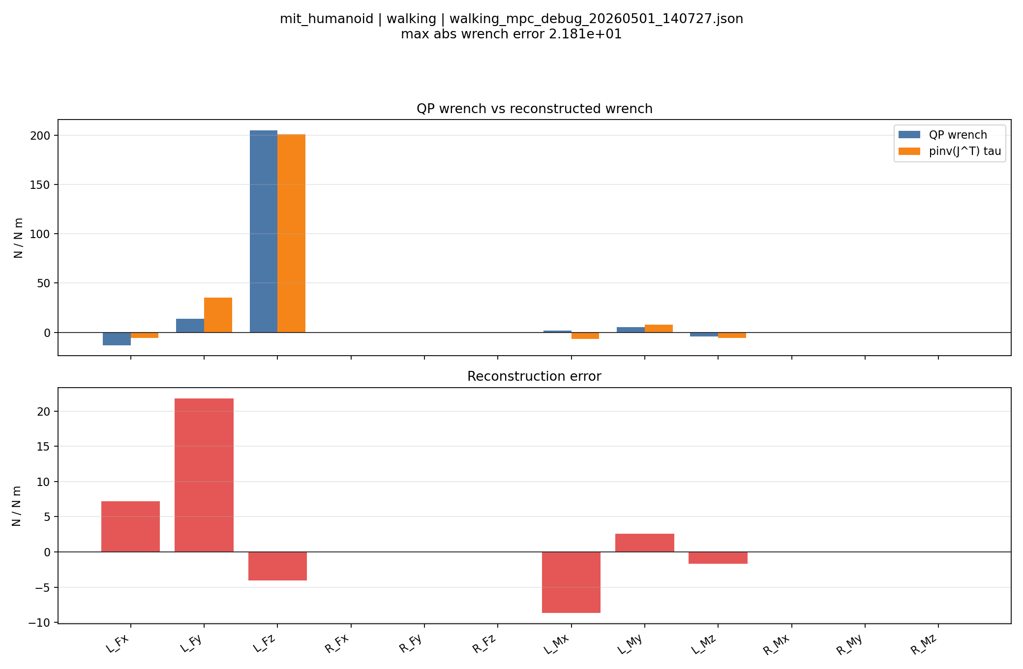
Stack a foot's Jacobians into $A = [J_v^\top\; J_\omega^\top]^\top$-adjoint form, mapping wrench to torque as $\boldsymbol{\tau} = A^\top \mathbf{w}$ with $A^\top \in \mathbb{R}^{n_j \times 6}$. For the MIT Humanoid, $n_j = 5$: the map cannot be injective, and there is (at least) a one-dimensional subspace of wrenches that produce zero joint torque — wrenches the leg simply cannot exert. What the leg actually realizes is the row-space projection

$$\mathbf{w}_{\mathrm{rec}} = \big(A^\top\big)^{+} \big(A^\top \mathbf{w}_{\mathrm{qp}}\big),$$

and the residual $\mathbf{w}_{\mathrm{qp}} - \mathbf{w}_{\mathrm{rec}}$ is silently discarded by physics. This is not hypothetical: with a pitch-only ankle, the missing DoF is essentially the ankle-roll moment, and any $M_x^F$ the QP requests evaporates at the torque map. Two design consequences follow. First, the no_roll_moment equality row of §5.6 exists so the QP knows about the null direction instead of spending wrench budget there. Second, the wrench-reconstruction probe of §12 computes exactly this projection from logged data, turning "the QP asked for something impossible" from a hunch into a plotted, per-axis error bar. On the 6-DoF-per-leg Unitree G1 the same machinery runs with the full wrench model and the equality row disabled — one YAML switch, no code change.

10Solver Engineering

A 500 Hz control loop with a 71 Hz QP leaves roughly a dozen milliseconds of budget per solve — including building the problem. The solver is OSQP through the OsqpEigen interface (ADMM, warm-startable, polish off, 200-iteration cap, adaptive $\rho$); the engineering is in what gets rebuilt, what gets reused, and what never gets materialized at all.

10.1 Shape of the problem

Table 4QP dimensions at $H = 25$.

Quantity	Expression	Size
Decision variables (wrench horizon)	$12H$	300
Inequality rows (friction + CoP + bounds)	$24H$	600
Equality rows (swing-zero / no-roll)	$12H$	300
Hessian	$12H \times 12H$, dense	300 × 300
Constraint matrix	$36H \times 12H$, block-sparse	900 × 300, ~1.6% dense

The Hessian $\mathbf{H} = 2(B_{\mathrm{qp}}^\top L B_{\mathrm{qp}} + K)$ is genuinely dense — condensing trades constraint sparsity for a small dense Hessian, and at 300×300 that is the right trade. The constraint matrix is the opposite: overwhelmingly structural zeros, and everything below is about never touching them.

10.2 Row-level sparsity that survives yaw rotation

OSQP updates matrix values cheaply but treats a changed sparsity pattern as a new problem requiring full re-setup. So the pattern is designed once, as the union of every nonzero any runtime state can produce — and the subtlety is that the yaw rotation of §5.5 changes which entries are nonzero. A friction row in the foot frame touches $\{F_x, F_z\}$; after rotation it touches $\{F_x, F_y, F_z\}$. A CoP row grows from $\{F_z, M_x\}$ to $\{F_z, M_x, M_y\}$. The committed pattern is therefore row-level:

Table 5Per-row sparse pattern for one foot's inequality block, in local wrench columns $\{F_x, F_y, F_z, M_x, M_y, M_z\}$.

Rows	Constraint	Pattern
0–3	Friction pyramid	$\{F_x, F_y, F_z\}$
4–5	Normal-force bounds	$\{F_z\}$
6–9	CoP polygon	$\{F_z, M_x, M_y\}$
10–11	Torsional friction	$\{F_z, M_z\}$

Equality rows are diagonal except the two no-roll slots, which reserve all three moment columns of their leg because the foot's $x$-axis rotates freely. A debug-build assertion sweeps every dense value against the committed pattern and throws if a future constraint would silently fall outside it — cheap insurance that has already paid for itself.

10.3 Direct fills, signatures, and warm starts

Three mechanisms keep the per-solve cost flat:

• Direct sparse fill. The dense $900\times300$ constraint matrix is never assembled. A value function maps (row, column) → coefficient straight from the per-step gait data — stance flags, foot yaws, foot axes — and the fill iterates once over the compressed sparse storage in order, writing each nonzero in place. The same in-order trick fills the Hessian's upper triangle. Assembly cost scales with the nonzero count, not the matrix area.
• Contact-signature cold starts. The stance/swing pattern across the horizon is hashed into a signature $(c_{L,k}, c_{R,k})_{k=1}^{H}$. Unchanged signature — the overwhelmingly common case — means the constraint structure is identical, and the solver takes the cheap path: update values, gradient, and bounds in place. A changed signature (a gait event entered or left the horizon window, or the contact manager overrode the near term) triggers a clean OSQP re-initialization, because warm-starting ADMM across a structural flip converges worse than starting cold.
• Shifted warm starts. Between solves with a stable signature, the previous solution is shifted one step — $\mathbf{u}^{\mathrm{ws}}_k = \mathbf{u}^\ast_{k+1}$, last step duplicated — matching how the horizon actually slides in time. If a solve still fails to converge, one retry runs from a fresh cold initialization before the controller treats it as a hard fault. Cold starts, signature changes, and retries are all counted and reported by the built-in profiler, so solver health is a number, not a feeling.

11A Robot-Independent Controller Core

Nothing in the controller core knows a joint ID, an actuator index, or a fixed joints-per-leg count. All robot specifics enter through two narrow interfaces, resolved once at startup:

• A RobotMujocoSpec — a small name-mapping class per robot that identifies the torso body, foot links and contact sites, leg and arm joint chains in the MJCF. Everything quantitative — masses, the body inertia tensor, joint/velocity/actuator indices, limb topology, foot Jacobians, reduced leg mass matrices and bias terms — is extracted from the MuJoCo model itself, never hand-copied into configuration.
• A per-robot YAML — gait timing, MPC weights and wrench model, swing and contact-manager tuning, command limits, initial pose. The controller reads it once at startup, and every MPC debug snapshot embeds the full parameter set, so a logged solve can always be traced to the exact tuning that produced it.

MIT Humanoid · 5-DoF legs · primary platform

Unitree G1 · 6-DoF legs · full-wrench model

Unitree H1 · integration target

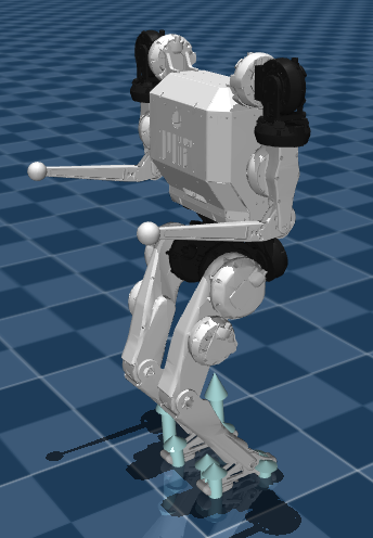
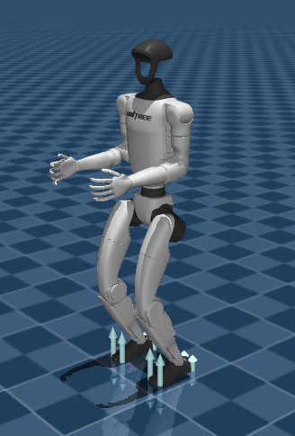
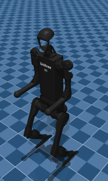
Figure 3Three humanoids, one controller. Runtime-sized limb data means the 5-DoF MIT leg and the 6-DoF G1 leg flow through identical code paths; the wrench model (full_wrench vs. no_roll_moment) is a YAML switch. The G1 and H1 configurations are integration starting points, not tuned results.

Adding a robot therefore requires exactly three artifacts — an MJCF model with assets, a RobotMujocoSpec mapping, and a YAML tuning file — plus registering the new RobotType. The discipline paid off immediately during development: bugs found on one robot were structural, not robot-specific, and fixes propagated for free.

12Reproducible Debugging: Four Layers of MPC Verification

An MPC controller fails in ways a PD controller cannot: the robot stumbles, and the cause might be the model, the reference, the constraints, the solver, or none of them — a torque map or a simulator disagreement downstream of a perfectly good solve. Staring at a live viewer does not localize such failures. The methodology here is a debugging principle made executable:

Principle

Every important MPC result must be reproducible from a captured controller state, offline, without the simulator running — and each potential failure layer must be testable in isolation.

Pressing Shift+L (or hitting a configured trigger time) captures the next scheduled solve as a self-contained JSON snapshot: the full MuJoCo qpos/qvel, the applied torque command, the reduced state $\mathbf{x}_0$, the reference trajectory and contact schedule, the condensed matrices $A_{\mathrm{qp}}, B_{\mathrm{qp}}$, the optimized wrench horizon, foot positions and Jacobians, and the complete controller configuration. One script then runs four independent analyses, each isolating a different layer of the pipeline.

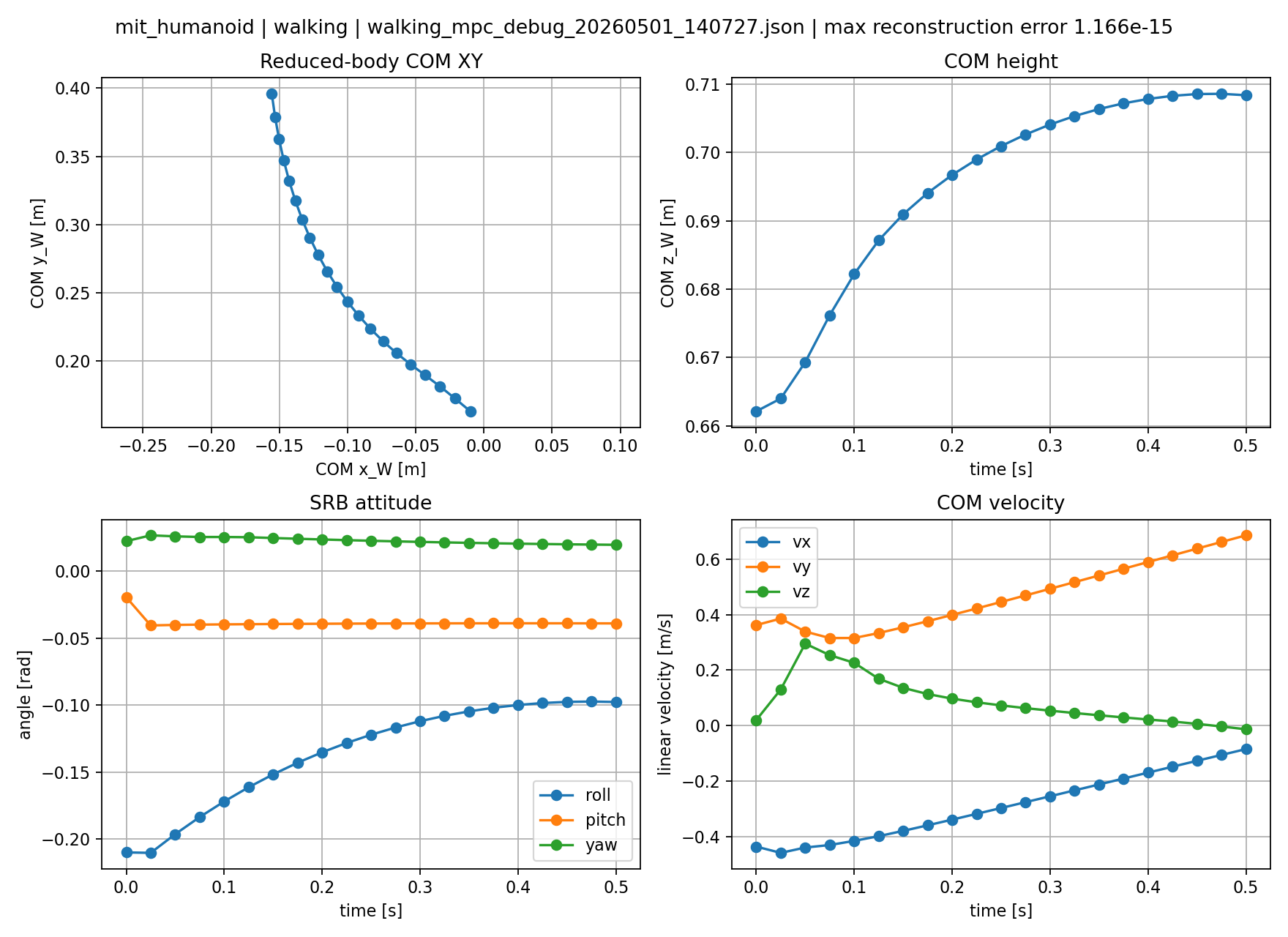
12.1 Layer 1 — SRB reconstruction: is the solve internally consistent?

Recompute the predicted horizon from the logged pieces, $\mathbf{X} = A_{\mathrm{qp}}\mathbf{x}_0 + B_{\mathrm{qp}}\mathbf{U}^\ast$, and compare against the stored prediction. This is a pure algebra check of the condensing and logging path — it must agree to machine precision, and it does (max reconstruction error ~$10^{-15}$). When it ever disagrees, the bug is in matrix assembly, not in control.

Figure 4SRB reconstruction of a captured walking solve: reconstructed COM path, height, attitude, and velocity horizon overlaid on the stored prediction. Agreement at $10^{-15}$ confirms the condensed algebra end-to-end.

12.2 Layer 2 — Wrench reconstruction: can the legs even do this?

Project the QP wrench through the leg-Jacobian row space, $\mathbf{w}_{\mathrm{rec}} = (A^\top)^{+}(A^\top \mathbf{w}_{\mathrm{qp}})$ (§9.3), and plot the per-axis residual. For the 5-DoF MIT leg this makes the unrealizable wrench directions visible as concrete error bars — the plot that motivated the no-roll-moment constraint and now guards it.

Figure 5QP wrench vs. its Jacobian row-space projection for one captured solve. Components that survive the projection are realizable by the leg; the residual (bottom) is what physics will silently discard.

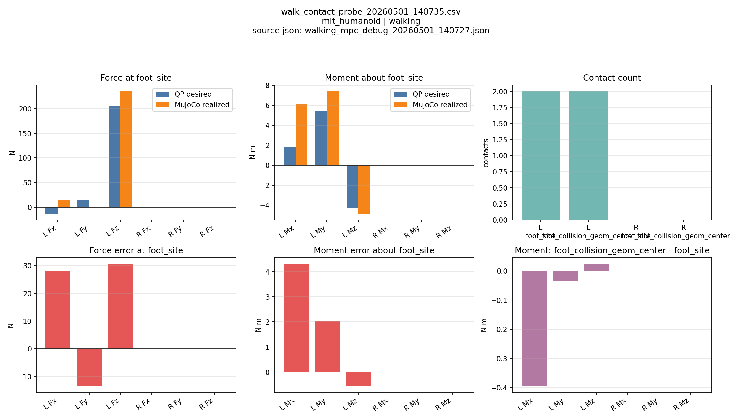
12.3 Layer 3 — MuJoCo contact probe: does the simulator agree?

Restore the exact logged state into MuJoCo, apply the recorded torque command, run mj_forward, and measure the realized contact wrench about the same reference point the controller used. This is the ground-truth arbiter for sign conventions, moment reference points, and controller/simulator frame agreement — the class of bug that produces plausible torques and inexplicable behavior.

Figure 6Contact probe: QP-desired vs. MuJoCo-realized force and moment at the stance foot, plus per-axis error and the sensitivity of the measured moment to the chosen reference point.

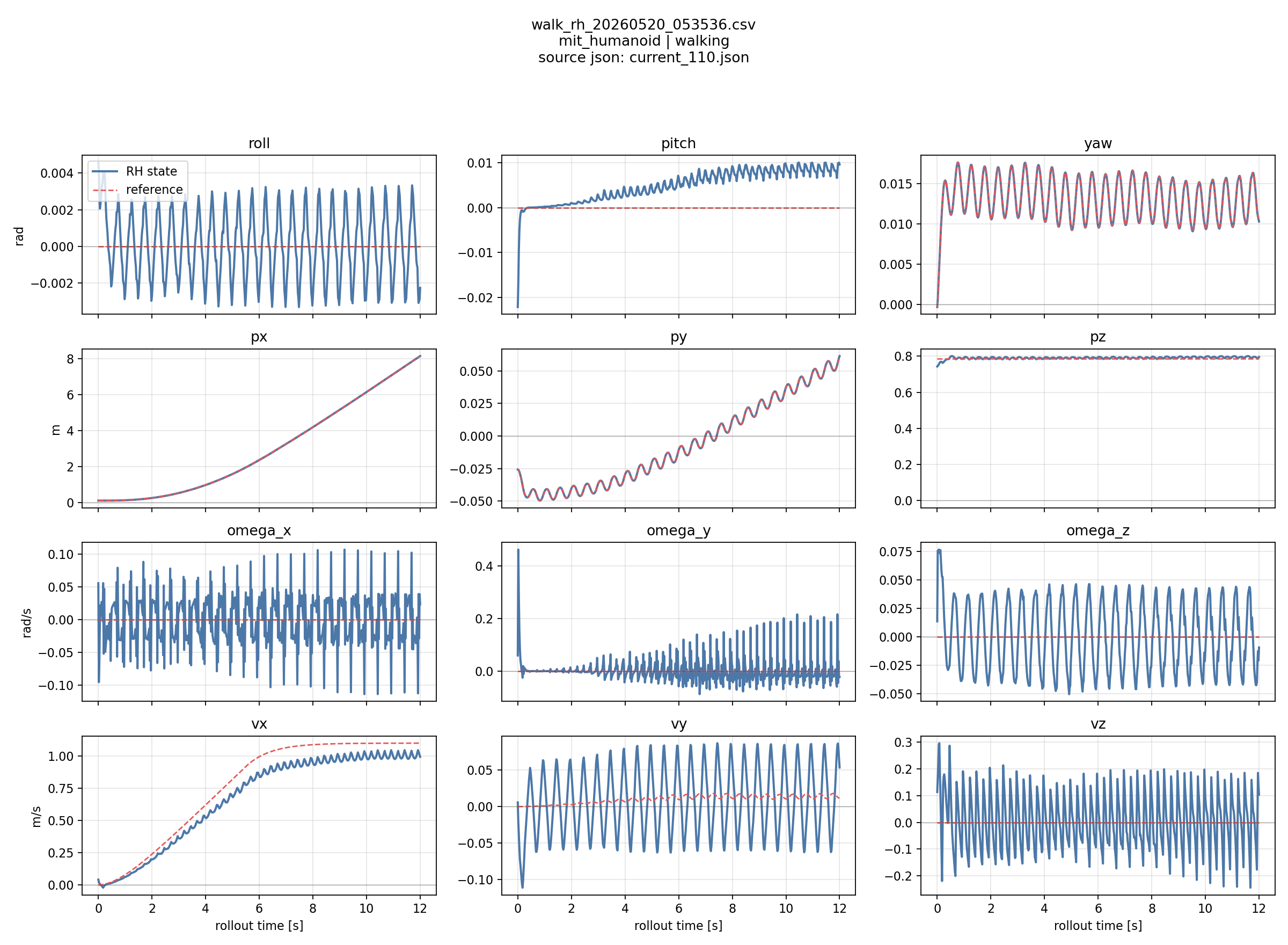
12.4 Layer 4 — Receding-horizon replay: does the loop work?

Starting from the captured state, rebuild reference, gait constraints, foot targets, SRB formulation, and QP at every rollout step — then propagate the ideal SRB model with each solve's first input. This is the controller running closed-loop against its own model, isolated from MuJoCo: reference tracking, contact-schedule updates, wrench evolution, and horizon-to-horizon consistency, all offline, with command sweeps (e.g. ramping $\dot x_{\mathrm{cmd}}$) available as flags. Divergence here is a formulation problem; convergence here plus failure in simulation points the finger at the layers below.

Figure 7Receding-horizon replay over 12 s (~860 re-solves): all twelve reduced states tracking their references through a commanded forward-velocity ramp to 1 m/s under the gait's periodic contact switching.

12.5 Live telemetry: shared memory to the browser

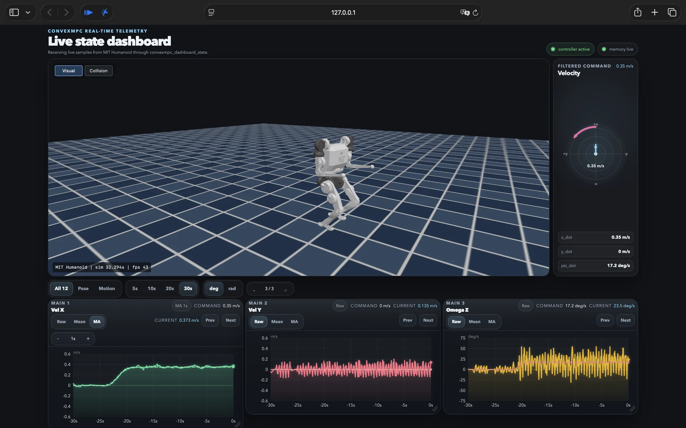
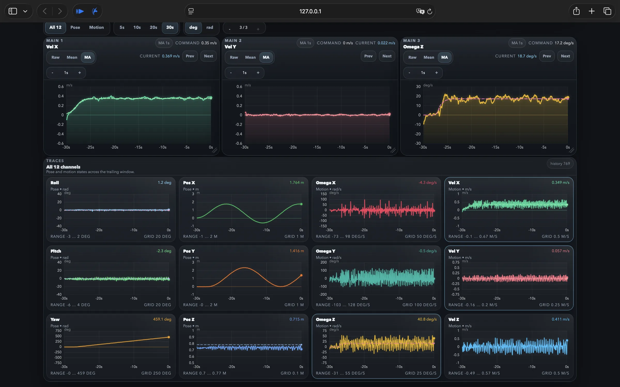
For interactive work, the controller publishes state and telemetry through shared memory to a Python-served web dashboard: twelve controller state channels with command overlays, a command compass, draggable multi-chart layouts — and a MuJoCo-WASM viewer that renders the same MJCF model from streamed qpos, so the browser shows the robot the controller believes in. The C++ side never blocks on a socket: C++ → shared memory → Python → browser.

Figure 8The web dashboard: live MuJoCo-WASM viewer with filtered-command compass (left), and the twelve-channel telemetry grid with per-chart raw/mean/moving-average modes (right).

13Results

All results below are the MIT Humanoid in MuJoCo at 500 Hz physics, running the single controller and single weight set documented throughout this article — no per-behavior mode switching beyond the standing/walking FSM. The clips show commanded operating points, not envelope maxima.

Forward · $\dot x = 0.6$ m/s

Lateral · $\dot y = 0.3$ m/s

In-place turn · $\dot\psi = 1.3$ rad/s

Roll tracking · $|\phi| \le 30°$

Pitch tracking · $|\theta| \le 30°$

Height tracking · $p_z$ command

Video 2Locomotion and body-pose tracking under one controller: omnidirectional walking, in-place turning at 1.3 rad/s, and standing-mode roll/pitch/height tracking. The combined demonstration is Video 1 at the top of the article.

13.1 The numbers behind the clips

Table 6MIT Humanoid operating configuration (all YAML-driven).

Parameter	Value
Gait cycle / swing / stance	0.5 s / 0.17 s / 0.33 s
Double-support fraction	32% of cycle
Horizon	25 steps × 20 ms = 0.5 s (one full cycle)
MPC solve cadence	every 7 ticks ≈ 71.4 Hz
Command limits $(\dot x, \dot y, \dot\psi)$	0.7 m/s, 0.5 m/s, 2.0 rad/s
Friction $\mu$ / torsional scale	1.0 / 0.0657
Foot half-length $a$ / half-width $b$	6.5 cm / 1.0 cm
Normal force bounds	$5 \le F_z \le 1500$ N
Swing height / natural frequency	6 cm / (151, 151, 110) rad/s

Table 7Walking-mode MPC weights (diagonal of $Q$; input weight $R = 10^{-3}\,\mathbf{1}_{12}$). The heavy planar-position and height weights — with $p_y$ five times $p_x$ — are what the body-yaw cost transform of §4.3 keeps pointed at the robot's actual lateral axis while turning.

$\phi$	$\theta$	$\psi$	$p_x$	$p_y$	$p_z$	$\omega_{x,y,z}$	$v_x$	$v_y$	$v_z$
5·10⁴	9·10³	500	2·10⁵	~10⁶	1.1·10⁵	10	100	70	10

Two qualitative observations from tuning that the tables cannot show. First, the CoP constraints are not decorative: widening the modeled foot beyond its physical dimensions produces immediate foot-roll at touchdown, and narrowing it makes the QP visibly re-route moment demand into tangential force pairs — the constraint set is active and load-bearing in ordinary walking. Second, the contact manager earns its complexity at the transitions: with early-contact handling disabled, small terrain-timing mismatches that the schedule cannot see accumulate into stumbles within a few strides; with it enabled, the same mismatches are absorbed as single-tick target freezes that are hard to even spot in the viewer.

14Limitations and Future Work

Being precise about what this project does not do is part of doing it honestly:

• Ground-truth state estimation. The estimator is cheater-state: exact body pose and twist from the simulator. Every result inherits that assumption. Sensor-based estimation (IMU + kinematics fusion) is the first prerequisite for any hardware claim, and the architecture reserves the seam for it — the controller consumes a StateEstimate interface, not simulator internals.
• Flat ground only. Touchdown targets assume a horizontal plane at $z = 0$; the yaw-only foot frame of §5 assumes level contact. Uneven terrain needs terrain-adaptive foot placement and a contact frame with full orientation.
• Velocity tracking, weak absolute position. The receding reference design (§6) deliberately forgets world position, so drift is unregulated by construction. A loose outer position loop feeding velocity commands is the natural extension for waypoint behaviors.
• Modest speed envelope. The validated gait is conservative (32% double support, 0.7 m/s command cap). Faster walking wants gait-timing adaptation and likely a flight-capable schedule, neither attempted here.
• Tuning maturity. The MIT Humanoid configuration is validated; the Unitree G1/H1 configurations are integration scaffolding awaiting robot-specific tuning passes.

The near-term roadmap follows directly: sensor-based state estimation, terrain-adaptive foothold selection, and hardware validation — in that order, because each is a precondition for honestly attempting the next.

15Closing Thoughts

The Cheetah 3 paper's deepest claim was never about quadrupeds — it was that a drastically simplified model, solved exactly and fast, beats a faithful model solved slowly and approximately. This project is an extended test of that claim on a much less forgiving platform, and the claim survives — provided the simplifications are chosen with care at the interfaces. The SRB model did not need to become nonlinear to walk a biped; it needed honest constraints (§5), an honest cost frame (§4.3), honest contact bookkeeping (§7), and honest accounting of what the legs can actually do (§9.3). Every one of those adjectives was earned by a specific failure, and nearly every failure was found by the debugging discipline of §12 rather than by staring at a falling robot.

If a single lesson carries beyond this codebase: make the optimizer's beliefs inspectable. A convex QP will always give you the exactly-optimal answer to the question you asked; the engineering is in noticing, quickly and reproducibly, when you asked the wrong question.

16References

1. J. Di Carlo, P. M. Wensing, B. Katz, G. Bledt, and S. Kim, “Dynamic Locomotion in the MIT Cheetah 3 Through Convex Model-Predictive Control,” IEEE/RSJ International Conference on Intelligent Robots and Systems (IROS), 2018.
2. J. Li and Q. Nguyen, “Force-and-Moment-Based Model Predictive Control for Achieving Highly Dynamic Locomotion on Bipedal Robots,” IEEE Conference on Decision and Control (CDC), 2021.
3. M. H. Raibert, Legged Robots That Balance, MIT Press, 1986.
4. B. Stellato, G. Banjac, P. Goulart, A. Bemporad, and S. Boyd, “OSQP: an operator splitting solver for quadratic programs,” Mathematical Programming Computation, 12(4), 2020.
5. E. Todorov, T. Erez, and Y. Tassa, “MuJoCo: A physics engine for model-based control,” IROS, 2012.

Written by Inseong Paik · June 2026. The full implementation — controller, simulator harness, debugging tools, and web dashboard — is available at github.com/ispaik06/convex-mpc-biped. The MIT Humanoid model files are not redistributed. Mathematical notation follows the conventions of the technical notes in the repository's docs/ directory, which contain longer-form derivations of the constraint matrices, yaw policy, gait scheduling, and reference trajectory described here. Math is pre-rendered with KaTeX; no external resources are loaded at view time.